Oscillators & State Space Systems

Modal Analysis

Oscillators are coupled mass/spring, pendulums, etc systems, which can be analysed using modal analysis:

• Start with a complex coupled system
• Use spectral decomposition to diagonalise the system into simpler uncoupled systems
• Solve for each system

Single Degree of Freedom Oscillators

Mass-Spring

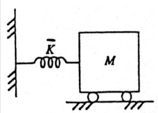
The equation of motion is:

$$\frac{d^{2}z(t)}{d{t}^2}=-kz(t)$$

where $k$ is the normalised stiffness, $k=\bar{k}/m$. Assuming an oscillatory solution:

$$z(t)=A\cos {\omega }_{0}t+B\sin {\omega }_{0}t$$ $$\dot{z}(t)=-{\omega }_{0}A\sin {\omega }_{0}t+{\omega }_{0}B\cos {\omega }_{0}t$$ $$\ddot{z}(t)=-{\omega }_0^{2}A\cos {\omega }_{0}t-{\omega }_0^{2}B\sin {\omega }_{0}t$$

Solving for ${\omega }_0$ by substituting back in gives ${\omega }_0=\sqrt{k}$.

Setting $z(0)=0$ and $\dot{z}(0)=v_0$:

$$z(t)=a\sin ({\omega }_{0}t)a=\frac{v_0}{{\omega }_0}$$

This system oscillates at a single frequency, ${\omega }_0=\sqrt{\bar{k}/m}$.

Pendulum

The equation of motion for a pendulum in the tangential direction is:

$$ml\ddot{\theta }=-mg\sin \theta$$ $$\ddot{\theta }(t)=-k\theta (t)\text{(for small}\theta \text{)}$$

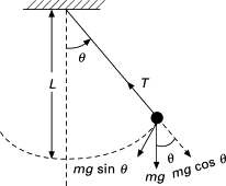
Where $k=g/l$

• The system oscillates at the frequency ${\omega }_0=\sqrt{k}$
• This system has the same form, and therefore solution, as the mass-spring.
• The frequency depends only on the length, not the mass, a property unique to pendulums.

Multiple Degrees of Freedom

This single degree of freedom can be generalised to a 2nd order $n$-degree of freedom system:

$$\frac{d^{2}y}{d{t}^2}=-Ky(t)$$

$$K=\left[\begin{array}{cccc}{k}_{11}& k_{12}& \dots & k_{1n}\\ k_{21}& k_{22}& \dots & k_{2n}\\ ⋮& ⋮& \ddots & ⋮\\ k_{n1}& k_{n2}& \dots & k_{nn}\end{array}\right]y=\left[\begin{array}{c}{y}_1\\ y_2\\ ⋮\\ y_n\end{array}\right]$$

• $K$ is an $n\times n$ matrix
• $y$ is an $n$-dimensional column vector

The goal is to find frequencies $\omega$ such that the solution $y(t)$ can be expressed as harmonic functions of $\sin (\omega t)$. This is done by spectral decomposition:

$$K=V\Lambda V^{-1}$$ $$\frac{d^{2}y}{d{t}^2}=-V\Lambda V^{-1}y(t)$$ $$\frac{d^2{V}^{-1}y}{d{t}^2}=-V^{-1}V\Lambda V^{-1}y(t)$$

Introduce a new variable $z(t)=V^{-1}y(t)$, so that for $z(t)$:

$$\frac{d^{2}z}{d{t}^2}=-\Lambda z(t)$$

$$\Lambda =\left[\begin{array}{cccc}{\lambda }_1& 0& \dots & 0\\ 0& {\lambda }_2& \dots & 0\\ ⋮& ⋮& \ddots & ⋮\\ 0& 0& \dots & {\lambda }_n\end{array}\right]$$

This equation involving a diagonal matrix can then be decomposed to $n$ uncoupled scalar equations (the normal modes) for each scalar $z_i$ in $z$:

$$\frac{d^2{z}_i}{d{t}^2}=-{\lambda }_{i}z(t)$$

This is a single degree of freedom scalar equation, as the previous two examples, thus:

• ${\lambda }_i={\omega }_i^2$
• $z(t)=a\sin (\omega t)$

The solution of the 2nd order $n$-DoF system is defined by a superposition of the normal modes $z_i(t)$

• ${\lambda }_i={\omega }_i^2$ is an eigenvalue of $K$
  • ${\omega }_i$ is the frequency of the normal mode
• $v_i$ is an eigenvector of $K$
  • Specifies the shape of the normal mode

Example 1

Conside a system of two coupled masses:

• Two masses $m_1$ and $m_2$
• Two displacements $y=\left[\begin{array}{c}{y}_1\\ y_2\end{array}\right]$
  • The variable to solve for
• Three springs $k_1$, $k_2$, $k_3$

Two equations of motion, one for each mass:

$$m_1\frac{d^2{y}_1}{d{t}^2}=-k_1{y}_1-k_3(y_1-y_2)$$ $$m_2\frac{d^2{y}_2}{d{t}^2}=-k_2{y}_2+k_3(y_1-y_2)$$

Rearranging into a matrix equation:

$$\frac{d^2{y}_1}{d{t}^2}=\frac{-(k_1+k_3)y_1+k_3{y}_2}{m_1}$$ $$\frac{d^2{y}_2}{d{t}^2}=\frac{k_3{y}_1-(k_3+k_3)y_2}{m_2}$$

$$\frac{d^{2}y}{d{t}^2}=-\left[\begin{array}{cc}\frac{k_1+k_3}{m_1}& \frac{-k_3}{m_1}\\ \frac{-k_3}{m_2}& \frac{k_2+k_3}{m_2}\end{array}\right]\left[\begin{array}{c}{y}_1\\ y_2\end{array}\right]=-Ky$$

Let $k_1=k_2=2$, and $k_3=m_1=m_2=1$:

$$K=\left[\begin{array}{cc}3& -1\\ -1& 3\end{array}\right]$$

To solve the system, need to compute the eigenvalues and eigenvectors of $K$, and hence the normal modes. Starting with the eigenvalues:

$$\left|\begin{array}{cc}3-\lambda & -1\\ -1& 3-\lambda \end{array}\right|=0$$

$${\lambda }^2-6\lambda +8=0$$ $${\lambda }_1=2{\lambda }_2=4$$

Hence the two natural frequencies of oscillation are ${\omega }_1=\sqrt{2}$ and ${\omega }_2=2$. Now for the eigenvectors:

$$(A-{\lambda }_i)v=0$$

$${\lambda }_1=2\left[\begin{array}{cc}1& -1\\ -1& 1\end{array}\right]\left[\begin{array}{c}{v}_1^{(1)}\\ v_2^{(2)}\end{array}\right]=0$$

$$v_1^{(1)}=v_2^{(2)}$$

$$v^{(1)}=\left[\begin{array}{c}1\\ 1\end{array}\right]$$

$${\lambda }_2=4\left[\begin{array}{cc}-1& -1\\ -1& -1\end{array}\right]\left[\begin{array}{c}{v}_1^{(1)}\\ v_2^{(2)}\end{array}\right]=0$$

$$v_1^{(1)}=-v_2^{(2)}$$

$$v^{(1)}=\left[\begin{array}{c}1\\ -1\end{array}\right]$$

The first mode ${\lambda }_1=2$, $v^{(1)}=\left[\begin{array}{c}1\\ 1\end{array}\right]$, ${\omega }_1=\sqrt{2}$ implies that both bodies move in unison at the frequency of the mode f = \frac{1}{\sqrt{2\pi}Hz. The spring between the two masses does not stretch or contract.

The second mode ${\lambda }_1=4$, $v^{(2)}=\left[\begin{array}{c}1\\ -1\end{array}\right]$, ${\omega }_2=2$ implies that both bodies move in opposition at the frequency of the mode $f=\frac{1}{\pi }$Hz, with the connecting spring stretching and contracting.

Example 2

The full nonlinear equations of motion for a double pendulum are:

$$(m_1+m_2)L_1\ddot{{\theta }_1}+m_2{L}_2\dot{{\theta }_2^2}\sin ({\theta }_1-{\theta }_2)+m_2{L}_2\ddot{{\theta }_2}\cos ({\theta }_1-{\theta }_2)+(m_1+m_2)g\sin ({\theta }_1)=0$$ $$m_2{L}_2\ddot{{\theta }_2}+m_2{L}_1\ddot{{\theta }_1}\cos ({\theta }_1-{\theta }_2)-m_2{L}_1\dot{{\theta }_1^2}\sin ({\theta }_1-{\theta }_2)+m_{2}g\sin {\theta }_2$$

Assuming small angles, and therefore neglecting square terms and making small angle trigonometric approximations:

$$(m_1+m_2)L_1\ddot{{\theta }_1}+m_2{L}_2\ddot{{\theta }_2}+(m_1+m_2)g{\theta }_1=0$$ $$m_2{L}_2\ddot{{\theta }_2}+m_2{L}_1\ddot{{\theta }_1}+m_{2}g{\theta }_2=0$$

Let:

• $m_1=1$
• $m_2=5$
• $L_1=2$
• $L_2=3$

$$12\ddot{{\theta }_1}+15\ddot{{\theta }_2}+60{\theta }_1=0$$ $$10\ddot{{\theta }_2}+15\ddot{{\theta }_1}+50{\theta }_2=0$$

$$\left[\begin{array}{cc}12& 15\\ 10& 15\end{array}\right]\left[\begin{array}{c}\ddot{{\theta }_1}\\ \ddot{{\theta }_2}\end{array}\right]+\left[\begin{array}{cc}60& 0\\ 0& 50\end{array}\right]\left[\begin{array}{c}{\theta }_1\\ {\theta }_2\end{array}\right]=0$$

$$\left[\begin{array}{cc}12& 15\\ 10& 15\end{array}\right]\left[\begin{array}{c}\ddot{{\theta }_1}\\ \ddot{{\theta }_2}\end{array}\right]=-\left[\begin{array}{cc}60& 0\\ 0& 50\end{array}\right]\left[\begin{array}{c}{\theta }_1\\ {\theta }_2\end{array}\right]$$

To put into the form $\ddot{\theta }=-K\theta$, we can premultiply by the inverse of the first matrix:

$$\left[\begin{array}{c}\ddot{{\theta }_1}\\ \ddot{{\theta }_2}\end{array}\right]=-{\left[\begin{array}{cc}12& 15\\ 10& 15\end{array}\right]}^{-1}\left[\begin{array}{cc}60& 0\\ 0& 50\end{array}\right]\left[\begin{array}{c}{\theta }_1\\ {\theta }_2\end{array}\right]$$

$$\left[\begin{array}{c}\ddot{{\theta }_1}\\ \ddot{{\theta }_2}\end{array}\right]=-\left[\begin{array}{cc}30& -25\\ -20& 20\end{array}\right]\left[\begin{array}{c}{\theta }_1\\ {\theta }_2\end{array}\right]$$

Now we have $K$, we can compute it's normal modes.

Mode 1 ${\lambda }_1$:

• ${\lambda }_1=2.0871$
• ${\omega }_1=1.4447$ rad/s
  • The system oscillates at a low frequency
• $v^{(1)}=\left[\begin{array}{c}0.6672\\ 0.7449\end{array}\right]$
  • System oscillates in-phase

Mode 2 ${\lambda }_2$:

• ${\lambda }_2=47.9129$
• ${\omega }_1=6.9219$ rad/s
  • The system oscillates at a high frequency
• $v^{(1)}=\left[\begin{array}{c}0.8129\\ -0.5824\end{array}\right]$
  • System oscillates out of phase

The oscillation of the overall system will be the superposition of these two modes.

State Space Linear Systems

Consider a second order linear ODE of the form $\ddot{y}(t)+a\dot{y}(t)+by(t)=0$. Two variables are needed to uniquely specify the state of the system at any moment in time, the displacement $x_1=y(t)$, and the velocity $x_2=\dot{y}(t)$. The system can be rewritten in terms of these:

$$\dot{x_1}=\dot{y}=x_2$$ $$\dot{x_2}=\ddot{y}=-a\dot{y}-by=-a{x}_2-b{x}_1$$

$$\left[\begin{array}{c}\dot{x_1}\\ \dot{x_2}\end{array}\right]=\left[\begin{array}{cc}0& 1\\ -b& -a\end{array}\right]\left[\begin{array}{c}{x}_1\\ x_2\end{array}\right]$$

This has replaced a 2nd order scalar equation with a two-state 1st order matrix equation. This concept can be generalised to express an $n$th order linear ODE as an $n$-state first order linear matrix ODE:

$$\left[\begin{array}{c}\dot{x_1}\\ \dot{x_2}\\ ⋮\\ \dot{x_n}\end{array}\right]=\left[\begin{array}{ccccc}0& 1& 0& \dots & 0\\ 0& 0& 1& \dots & 0\\ ⋮& ⋮& ⋮& \ddots & ⋮\\ 0& 0& 0& \dots & 1\\ -a_n& -a_{n-1}& -a_{n-2}& \dots & -a_1\end{array}\right]\left[\begin{array}{c}{x}_1\\ x_2\\ ⋮\\ x_n\end{array}\right]$$

Where the state vector $x(t)={\left[\begin{array}{cccc}{x}_1& x_2& \dots & x_n\end{array}\right]}^{\prime }$

• $x_1=y$
• $x_2=y^{\prime }=\dot{x_1}$
• $x_3=y^{\prime \prime }=\dot{x_2}$
• $x_n=y^{(n)}=\dot{x_{n-1}}$

Now to work out how to solve it. In the scalar case, the solution to $\dot{x}(t)=ax(t)$ with $x(0)=0$ has the form

$$x(t)=e^{at}{x}_0=x_0(1+at+\frac{(at{)}^2}{2!}+\frac{(at{)}^3}{3!}+\dots )$$

The sign of $a$ determines the stability of the system:

• $a$ is negative: the system decays exponentially and is stable
• $a$ is zero: nothing ever happens
• $a$ is positive: the system rises exponentially and is unstable

The matrix case has the same solution:

$$x(t)=e^{At}{x}_0=x_0(I_n+At+\frac{(At{)}^2}{2!}+\frac{(At{)}^3}{3!}+\dots )$$

The task is then to compute the matrix exponential, and characterise the dynamics of the solution using the matrix $A$.

Suppose $A$ has the spectral decomposition $A=V\Lambda V^{-1}$:

$$\dot{x}(t)=Ax(t)=V\Lambda V^{-1}x(t)$$ $$\dot{x}(t)=Ax(t)=\Lambda V^{-1}x(t)$$

Defining $z(t)=V^{-1}x(t)$ again:

$$\dot{z}(t)=\Lambda z(t)$$

$$z(t)=\left[\begin{array}{cccc}{e}^{{\lambda }_{1}t}& 0& \dots & 0\\ 0& e^{{\lambda }_{2}t}& \dots & 0\\ ⋮& ⋮& \ddots & ⋮\\ 0& 0& \dots & e^{{\lambda }_{n}t}\end{array}\right]z(0)$$

Since $\Lambda$ is diagonal, this is now a set of uncoupled equations:

$$\dot{z_1}(t)={\lambda }_1{z}_1(t)⟹z_1(t)=e^{{\lambda }_{1}t}{z}_1(0)$$ $$\dot{z_2}(t)={\lambda }_1{z}_2(t)⟹z_2(t)=e^{{\lambda }_{1}t}{z}_2(0)$$ $$\dot{z_n}(t)={\lambda }_1{z}_n(t)⟹z_n(t)=e^{{\lambda }_{1}t}{z}_n(0)$$

$z_1(t),z_2(t),\dots ,z_n(t)$ are the individual modes of the solution $x(t)$ and are defined by the eigenvalues ${\lambda }_1,{\lambda }_2,\dots ,{\lambda }_n$ alone. The matrix exponential $e^{At}$ is given by:

$$e^{At}=Vz(t)=V\mathrm{diag}\{e^{{\lambda }_{1}t},e^{{\lambda }_{2}t},\dots ,e^{{\lambda }_{n}t\}}{V}^{-1}$$

Multiplying by the starting state $x(0)=x_0$ gives:

$$x(t)=x_0{e}^{At}=x_{0}V\mathrm{diag}\{e^{{\lambda }_{1}t},e^{{\lambda }_{2}t},\dots ,e^{{\lambda }_{n}t\}}{V}^{-1}$$

• The solution is a linear combination of the terms $e^{{\lambda }_{1}t},e^{{\lambda }_{2}t},\dots ,e^{{\lambda }_{n}t}$
• Hence, behaviour is defined by the eigenvalues
• The system is stable if all eigenvalues are negative
• If at least one is positive, the system is unstable

Example

Consider an elementary RLC circuit with all components in series, with a non-zero initial charge $q_0$ on the capacitor. The instantaneous charge $q(t)$ in the circuit is described by a linear state space differential equation where $x(t)=\left[\begin{array}{c}q(t)\\ \dot{q}(t)\end{array}\right]$ and $x_0=\left[\begin{array}{c}{q}_0\\ 0\end{array}\right]$. Suppose:

• $q_0=6$
• $R=7$
• $L=1$
• $C=0.1$

Find the particular solution for this system and discuss it's stability.

The state space equation for the system in the form $\dot{x}(t)=Aq(t)$ is:

$$\left[\begin{array}{c}\dot{x_1}(t)\\ \dot{x_2}\end{array}\right]=\left[\begin{array}{cc}0& 1\\ -10& -7\end{array}\right]\left[\begin{array}{c}q(t)\\ \dot{q}(t)\end{array}\right]$$

The eigenvalues and eigenvectors of $A$ are:

$${\lambda }_1=-2v^{(1)}=\left[\begin{array}{c}1\\ -2\end{array}\right]$$

$${\lambda }_2=-5v^{(2)}=\left[\begin{array}{c}1\\ -5\end{array}\right]$$

The spectral resolution of $A$:

$$V=\left[\begin{array}{cc}1& 1\\ -2& -5\end{array}\right]$$

$$V^{-1}=-\frac{1}{3}\left[\begin{array}{cc}-5& -1\\ 2& 1\end{array}\right]$$

$$\Lambda =\left[\begin{array}{cc}-2& 0\\ 0& -5\end{array}\right]$$

$$A=-\frac{1}{3}\left[\begin{array}{cc}1& 1\\ -2& -5\end{array}\right]\left[\begin{array}{cc}-2& 0\\ 0& -5\end{array}\right]\left[\begin{array}{cc}-5& -1\\ 2& 1\end{array}\right]=\left[\begin{array}{cc}0& 1\\ -10& -7\end{array}\right]$$

The solution is given by $x(t)=e^{At}{x}_0$, and the matrix exponential term $e^{At}=V\mathrm{diag}\{e^{{\lambda }_{1}t},e^{{\lambda }_{2}t},\dots ,e^{{\lambda }_{n}t}\}{V}^{-1}$:

$$x(t)=\left[\begin{array}{cc}1& 1\\ -2& -5\end{array}\right]\left[\begin{array}{cc}{e}^{-2t}& 0\\ 0& e^{-5t}\end{array}\right]\left(\frac{-1}{3}\right)\left[\begin{array}{cc}-5& -1\\ 2& 1\end{array}\right]\left[\begin{array}{c}6\\ 0\end{array}\right]=\left[\begin{array}{c}-10e^{-2t}-4e^{-5t}\\ -20e^{-2t}+20e^{-5t}\end{array}\right]$$

Thus the solution:

$$q(t)=-10e^{-2t}-4e^{-5t}$$ $$\dot{q}(t)=-20e^{-2t}+20e^{-5t}$$

Also, since both eigenvalues $<0$, the system is stable.