Introduction
This book is a collection of all my notes from my degree (computer systems engineering).
It exists for a few purposes:
- To consolidate knowledge
- To aid revision
- To act as a reference during exams
Contributing
If you wish to contribute to this, either to make any additions or just to fix any mistakes I've made, feel free.
The sources are all available on my Github.
CS118
This section is mainly just a reference of some of the more detailed bits of the module. It assumes a pretty strong prior knowledge of object oriented programming so doesn't aim to be comprehensive, it just specifies some details to remember for the exam.
The version of Java on DCS systems at the time of writing is 11. This is also the version these notes refer to.
Useful Resources
- https://en.wikipedia.org/wiki/Single-precision_floating-point_format
- The Oracle documentation for specifics on how Java implements stuff
IEEE 754
IEEE 754 is a standardised way of storing floating point numbers with three components
- A sign bit
- A biased exponent
- A normalised mantissa
| Type | Sign | Exponent | Mantissa | Bias |
|---|---|---|---|---|
| Single Precision (32 bit) | 1 (bit 31) | 8 (bit 30 - 23) | 23 (bit 22- 0) | 127 |
| Double Precision (64 bit) | 1 (bit 63) | 11 (bit 62 - 52) | 52 (51 - 0) | 1023 |
The examples below all refer to 32 bit numbers, but the principles apply to 64 bit.
- The exponent is an 8 bit unsigned number in biased form
- To get the true exponent, subtract 127 from the binary value
- The mantissa is a binary fraction, with the first bit representing , second bit , etc.
- The mantissa has an implicit , so 1 must always be added to the mantissa
Formula
Decimal to Float
The number is converted to a binary fractional format, then adjusted to fit into the form we need. Take 12.375 for example:
- Integer part
- Fraction part
Combining the two parts yields . However, the standard requires that the mantissa have an implicit 1, so it must be shifted to the right until the number is normalised (ie has only 1 as an integer part). This yields . As this has been shifted, it is actually . The three is therefore the exponent, but this has to be normalised (+127) to yield 130 . The number is positive (sign bit zero) so this yields:
| Sign | Biased Exponent | Normalised Mantissa |
|---|---|---|
| 0 | 1000 0010 | 100011 |
Float to Decimal
Starting with the value 0x41C80000 = 01000001110010000000000000000000:
| Sign | Biased Exponent | Normalised Mantissa |
|---|---|---|
| 0 | 1000 0011 | 1001 |
- The exponent is 131, biasing (-127) gives 4
- The mantissa is 0.5625, adding 1 (normalising) gives 1.5625
- gives 25
Special Values
- Zero
- When both exponent and mantissa are zero, the number is zero
- Can have both positive and negative zero
- Infinity
- Exponent is all 1s, mantissa is zero
- Can be either positive or negative
- Denormalised
- If the exponent is all zeros but the mantissa is non-zero, then the value is a denormalised number
- The mantissa does not have an assumed leading one
- NaN (Not a Number)
- Exponent is all 1s, mantissa is non-zero
- Represents error values
| Exponent | Mantissa | Value |
|---|---|---|
| 0 | 0 | |
| 255 | 0 | |
| 0 | not 0 | denormalised |
| 255 | not 0 | NaN |
OOP Principles
Constructors
All Java classes have a constructor, which is the method called upon object instantiation.
- An object can have multiple overloaded constructors
- A constructor can have any access modifier
- Constructors can call other constructors through the
this()method. - If no constructor is specified, a default constructor is generated which takes no arguments and does nothing.
- The first call in any constructor is to the superclass constructor.
- This can be elided, and the default constructor is called
- If there is no default constructor, a constructor must be called explicitly
- Can call explicitly with
super()
- This can be elided, and the default constructor is called
Access Modifiers
Access modifiers apply to methods and member variables.
private: only the members of the class can seepublic: anyone can seeprotected: only class and subclasses can see- Default: package-private, only members of the same package can see
Inheritance
- To avoid the diamond/multiple inheritance problem, Java only allows for single inheritance
- This is done using the
extendskeyword in the class definition - Inherits all public and protected methods and members
- Can, however, implement multiple interfaces
Example:
public class Car extends Vehicle implements Drivable, Crashable{
// insert class body here
}
The Car class extends the Vehicle base class (can be abstract or concrete) and implements the behaviours defined by the interfaces Drivable and Crashable.
static
The static keyword defines a method, a field, or a block of code that belongs to the class instead of the object.
- Static fields share a mutable state accross all instances of the class
- Static methods are called from the class instead of from the object
- Static blocks are executed once, the first time the class is loaded into memory
Polymorphism
Polymorphism: of many forms. A broad term describing a few things in java.
Dynamic Polymorphism
An object is defined as polymorphic if it passes more than one instanceof checks. An object can be referred to as the type of any one of it's superclasses. Say for example there is a Tiger class, which subclasses Cat, which subclasses Animal, giving an inheritance chain of Animal <- Cat <- Tiger, then the following is valid:
Animal a = new Tiger();
Cat c = new Tiger();
Tiger t = new Tiger();
When referencing an object through one of it's superclass types, you can only call objects that the reference type implements. For example, if there was two methods, Cat::meow and Tiger::roar, then:
c.meow() //valid
t.meow() //valid
a.meow() //not valid - animal has no method meow
t.roar() //valid
c.roar() // not valid - cat has no method roar
Even though all these variables are of the same runtime type, they are being called from a reference of another type.
When calling a method of an object, the actual method run is the one that is furthest down the inheritance chain. This is dynamic/runtime dispatch.
public class Animal{
public speak(){return "...";}
}
public class Dog extends Animal{
public speak(){return "woof";}
}
public class Cat extends Animal{
public speak(){return "meow";}
}
Animal a = new Animal();
Animal d = new Dog();
Animal c = new Cat();
a.speak() // "..."
d.speak() // "woof"
c.speak() // "meow"
Even though the reference was of type Animal, the actual method called was the overridden subclass method.
Static Polymorphism (Method Overloading)
Note: different to overridding
- Multiple methods with the same name can be written, as long as they have different parameter lists
- The method that is called depends upon the number of and type of the arguments passed
Example:
public class Addition{
private int add(int x, int y){return x+y;}
private float add(float x, float y){return x+y;}
public static void main(String[] args){
add(1,2); //calls first method
add(3.14,2.72); //calls second method
add(15,1.5); //calls second method
}
}
Abstraction
Abstraction is the process of removing irrelevant details from the user, while exposing the relevant details. For example, you don't need to know how a function works, it's inner workings are abstracted away, leaving only the function's interface and details of what it does.
In the example below, the workings of the sine function are abstracted away, but we still know what it does and how to use it.
float sin(float x){
//dont care really
}
sin(90); // 1.0
Encapsulation
Encapsulation is wrapping the data and the code that acts on it into a single unit. The process is also known as data hiding, because the data is often hidden (declared private) behind the methods that retrieve them (getters/setters).
Reference Variables
There is no such thing as an object variable in Java. Only primitives (int,char,float...), and references. All objects are heap-allocated (new), and a reference to them stored. Methods are all pass by value: either the value of the primitive, or the value of the reference. Java is not pass by reference . Objects are never copied/cloned/duplicated implicitly.
If a reference type is required (ie Integer), but a primitive is given ((int) 1), then the primitive will be autoboxed into it's equivalent object type.
Abstract Classes and Interfaces
- Abstract classes are classes that contain one or more
abstractmethods.- A class must be declared
abstract - Abstract methods have no body, ie are unimplemented.
- The idea of them is to generalise behaviour, and leave it up to subclasses to implement
- Abstract classes cannot be instantiated directly, though can still have constructors for subclasses to call
- A class must be declared
- Interfaces are a special kind of class that contain only abstract methods (and fields declared
public static final)- Used to define behaviour
- Technically can contain methods, but they're default implementations
- This raises all sorts of issues so is best avoided
- Don't have to declare methods abstract, it's implicit
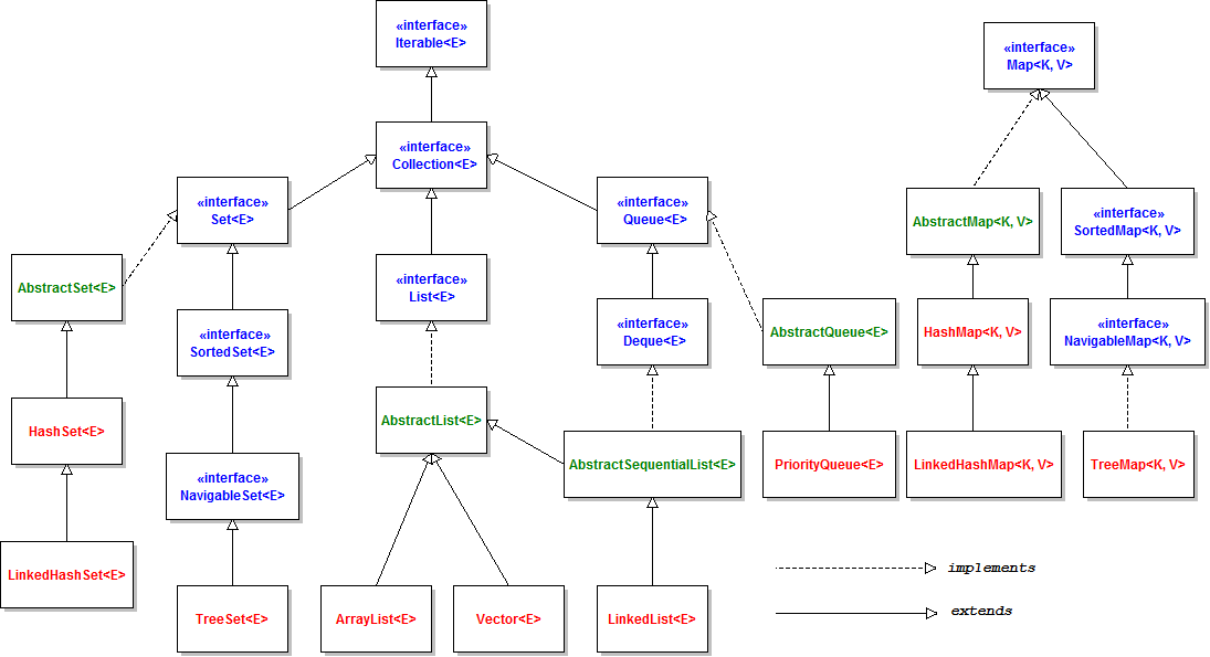
The diagram shows the inheritance hierarchy of the java collections framework, containing interfaces, abstract classes, and concrete classes.
Exceptions
Exceptions
Exceptions are events that occur within the normal flow of program execution that disrupt the normal flow of control.
Throwing Exceptions
Exceptions can occur when raised by other code we call, but an exception can also be raised manually using a throw statement. Any object that inherits, either directly or indirectly, from the Throwable class, can be raised as an exception.
//pop from a stack
public E pop(){
if(this.size == 0)
throw new EmptyStackException();
//pop the item
}
Exception Handling
- Exceptions can be caught using a
try-catchblock - If any code within the
tryblock raises an exception, thecatchblock will be executedcatchblocks must specify the type of exception to catch- Can have multiple catch blocks for different exceptions
- Only 1 catch block will be executed
- A
finallyblock can be included to add any code to execute after the try-catch, regardless of if an exception is raised or not. - The exception object can be queried through the variable
e
try{
//try to do something
} catch (ExceptionA e){
//if an exception of type ExceptionA is thrown, this is executed
} catch (ExceptionB e){
//if an exception of type ExceptionB is thrown, this is executed
} finally{
//this is always executed
}
Exception Heirachy
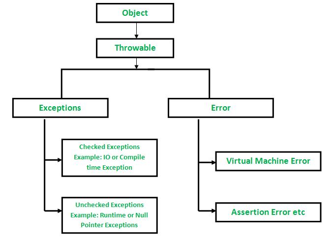
- The
Throwableclass is the parent class of all errors and exceptions in Java - There are two subclasses of
ThrowableError, which defines hard errors within the JVM that aren't really recoverableException, which defines errors that may occur within the code- There are two kinds of exception, checked and unchecked
Checked and Unchecked Exceptions
- Checked exceptions must be either caught or re-thrown
IOExceptionis a good example
- When a method that may throw a checked exception is required, there are two options
- Wrap the possibly exception-raising code in a
try-catch - Use the
throwskeyword in the method definition to indicate that the method may throw a checked exception
- Wrap the possibly exception-raising code in a
public static void ReadFile() throws FileNotFoundException{
File f = new File("non-existant-file.txt")
FileInputStream stream = new FileInputStream(f);
}
// OR
public static void ReadFile(){
File f = new File("non-existant-file.txt")
try{
FileInputStream stream = new FileInputStream(f);
} catch (FileNotFoundException){
e.printStackTrace();
return;
}
}
- Unchecked Exceptions all subclass
RunTimeException- ie
NullPointerExceptionandArrayIndexOutOfBoundsException
- ie
- Can be thrown at any point and will cause program to exit if not caught
Custom Exceptions
- Custom exception classes can be created
- Should subclass
Throwable- Ideally the most specific subclass possible
- Subclassing
Exceptiongives a new checked exception - Subclassing
RunTimeExceptiongives a new unchecked exception
- All methods such as
printStackTraceandgetMessageinherited from superclass - Should provide at least one constructor that overrides a superclass constructor
public class IncorrectFileExtensionException
extends RuntimeException {
public IncorrectFileExtensionException(String errorMessage, Throwable err) {
super(errorMessage, err);
}
}
Generics
Generics allow for classes to be parametrised over some type or types, to provide additional compile time static type checking. A simple box class parametrised over some type E, for example:
public class Box<E>{
E item;
public Box(E item){
this.item = item;
}
public E get(){
return item;
}
public E set(E item){
this.item = item;
}
}
Generic Methods
Methods can be generic too, introducing their own type parameters. The parameters introduced in methods are local to that method, not the whole class. As an example, the static method below compares two Pair<K,V> classes to see if they are equal.
public static <K, V> boolean compare(Pair<K, V> p1, Pair<K, V> p2) {
return p1.getKey().equals(p2.getKey()) &&
p1.getValue().equals(p2.getValue());
}
Type erasure
Type information in generic classes and methods is erased at runtime, with the compiler replacing all instances of the type variable with Object. Object is also what appears in the compiled bytecode. This means that at runtime, any type casting of generic types is unchecked, and can cause runtime exceptions.
CS126
The book Data Structures and Algorithms in Java by Goodrich, Tamassia and Goldwasser is a good resource as it aligns closely with the material. It can be found online fairly easily.
Arrays & Linked Lists
Arrays
Arrays are the most common data structure and are very versatile
- A sequenced collection of variables of the same type (homogenous)
- Each cell in the array has an index
- Arrays are of fixed length and so have a max capacity
- Can store primitives, or references to objects
- When inserting an element into the array, all to the right must be shifted up by one
- The same applies in reverse for removal to prevent null/0 gaps being left
Sorting Arrays
- The sorting problem:
- Consider an array of unordered elements
- We want to put them in a defined order
- For example
[3, 6, 2, 7, 8, 10, 22, 9]needs to become[2, 3, 6, 7, 8, 9, 10, 22]
- One possible solution: insertion sort:
- Go over the entire array, inserting each element at it's proper location by shifting elements along
public static void insertionSort(int[] data){
int n = data.length;
for(int k = 1; k < n; k++){ //start with second element
int cur = data[k]; //insert data[k]
int j = k; //get correct index j for cur
while(j < 0 && data[j-1] > cur){ //data[j-1] must go after cur
data[j] = data[j-1]; // slide data[j-1] to the right
j--; //consider previous j for cur
}
data[j] = cur; //cur is in the right place
}
}
- Insertion sort sucks
- Has worst case quadratic complexity, as k comparisons are required for k iterations.
- When the list is in reverse order (worst case), comparisons are made
- Can do much better with alternative algorithms
Singly Linked Lists
- Linked lists is a concrete data structure consisting of a chain of nodes which point to each other
- Each node stores the element, and the location of the next node
- The data structure stores the head element and traverses the list by following the chain
- Operations on the head of the list (ie, prepending) are efficient, as the head node can be accessed via its pointer
- Operations on the tail require first traversing the entire list, so are slow
- Useful when data needs to always be accessed sequentially
- Generally, linked lists suck for literally every other reason
Doubly Linked Lists
- In a doubly linked list, each node stores a pointer to the node in front of and behind it
- This allows the list to be traversed in both directions, and for nodes to be easily inserted mid-sequence
- Sometimes, special header and trailer "sentinel" nodes are added to maintain a reference to the head an tail of the list
- Also removes edge cases when inserting/deleting nodes as there is always nodes before/after head and tail
Analysis of Algorithms
This topic is key to literally every other one, and also seems to make up 90% of the exam questions (despite there being only 1 lecture on it) so it's very important.
- Need some way to characterise how good a data structure or algorithm is
- Most algorithms take input and generate output
- The run time of an algorithm typically grows with input size
- Average case is often difficult to determine
- Focus on the worst case
- Runtime analysis and benchmarks can be used to determine the performance of an algorithm, but this is often not possible
- Results will also vary from machine to machine
- Theoretical analysis is preferred as it gives a more high-level analysis
- Characterises runtime as a function of input size
Pseudocode
- Pseudocode is a high level description of an algorithm
- Primitive perations are assumed to take unit time
- For example
- Evaluating an expression
- Assigning to a variable
- Indexing into an array
- Calling a method
Looking at an algorithm, can count the number of operations in each step to analyse its runtime
public static double arrayMax(double[] data){
int n = data.length; //2 ops
double max = data[0]; //2 ops
for (int j=1; j < n;j++) //2n ops
if(data[j] > max) //2n-2 ops
max = data[j]; //0 to 2n-2 ops
return max; //1 op
}
- In the best case, there are primitive operations
- In the worst case,
- The runtime is therefore
- is the time to execute a primitive operation
Functions
There are 7 important functions that appear often when analysing algorithms
- Constant -
- A fixed constant
- Could be any number but 1 is the most fundamental constant
- Sometimes denoted where
- Logarithmic -
- For some constant ,
- Logarithm is the inverse of the power function
- Usually, because we are computer scientists and everything is base 2
- Linear -
-
- is a fixed constant
-
- n-log-n -
- Commonly appears with sorting algorithms
- Quadratic -
- Commonly appears where there are nested loops
- Cubic -
- Less common, also appears where there are 3 nested loops
- Can be generalised to other polynomial functions
- Exponential -
-
- is some arbitrary base, is the exponent
-
The growth rate of these functions is not affected by changing the hardware/software environment. Growth rate is also not affected by lower-order terms.
- Insertion sort takes time
- Characterised as taking time
- Merge sort takes
- Characterised as
- The
arrayMaxexample from earlier took time- Characterised as
- A polynomial of degree , is of order
Big-O Notation
- Big-O notation is used to formalise the growth rate of functions, and hence describe the runtime of algorithms.
- Gives an upper bound on the growth rate of a function as
- The statement " is " means that the growth rate of is no more than the growth rate of
- If is a polynomial of degree , then is
- Drop lower order terms
- Drop constant factors
- Always use the smallest possible class of functions
- is , not
- Always use the simplest expression
- is , not
Formally, given functions and , we say that is if there is a positive constant and a positive integer constant , such that
where , and
Examples
is :
The function is not The inequality does not hold, since must be constant.
Big-O of :
Big-O of :
is
Asymptotic Analysis
- The asymptotic analysis of an algorithm determines the running time big-O notation
- To perform asymptotic analysis:
- Find the worst-case number of primitive operations in the function
- Express the function with big-O notation
- Since constant factors and lower-order terms are dropped, can disregard them when counting primitive operations
Example
The th prefix average of an array is the average of the first elements of . Two algorithms shown below are used to calculate the prefix average of an array.
Quadratic time
//returns an array where a[i] is the average of x[0]...x[i]
public static double[] prefixAverage(double[] x){
int n = x.length;
double[] a = new double[n];
for(int j = 0; j < n; j++){
double total = 0;
for(int i = 0; i <= j; i++)
total += x[i];
a[j] = total / (j+1);
}
return a;
}
The runtime of this function is . The sum of the first integers is , so this algorithm runs in quadratic time. This can easily be seen by the nested loops in the function too.
Linear time
//returns an array where a[i] is the average of x[0]...x[i]
public static double[] prefixAverage(double[] x){
int n = x.length;
double[] a = new double[n];
double total = 0;
for(int i = 0; i <= n; i++){
total += x[i];
a[i] = total / (i+1);
}
return a;
}
This algorithm uses a running average to compute the same array in linear time, by calculating a running sum.
Big-Omega and Big-Theta
Big-Omega is used to describe the best case runtime for an algorithm. Formally, is if there is a constant and an integer constant such that
Big-Theta describes the average case of the runtime. is if there are constants and , and an integer constant such that
The three notations compare as follows:
- Big-O
- is if is asymptotically less than or equal to
- Big-
- is if is asymptotically greater than or equal to
- Big-
- is if is asymptotically equal to
Recursive Algorithms
Recursion allows a problem to be broken down into sub-problems, defining a problem in terms of itself. Recursive methods work by calling themselves. As an example, take the factorial function:
In java, this can be written:
public static int factorial(int n){
if(n == 0) return 1;
return n * factorial(n-1);
}
Recursive algorithms have:
- A base case
- This is the case where the method doesn't call itself, and the stack begins to unwind
- Every possible chain of recursive calls must reach a base case
- If not the method will recurse infinitely and cause an error
- A recursive case
- Calls the current method again
- Should always eventually end up on a base case
Binary Search
Binary search is a recursively defined searching algorithm, which works by splitting an array in half at each step. Note that for binary search, the array must already be ordered.
Three cases:
- If the target equals
data[midpoint]then the target has been found- This is the base case
- If the target is less than
data[midpoint]then we binary search everything to the left of the midpoint - If the target is greater than
data[midpoint]then we binary search everything to the right of the midpoint

public static boolean binarySearch(int[] data, int target, int left, int right){
if (left > right)
return false;
int mid = (left + right) / 2;
if(target == data[mid])
return true;
else if (target < data[mid])
return binarySearch(data,target,low,mid-1);
else
return binarySearch(data,target,mid+1,high);
}
Binary search has , as the size of the data being processed halves at each recursive call. After the call, the size of the data is at most .
Linear Recursion
- The method only makes one recursive call
- There may be multiple possible recursive calls, but only one should ever be made (ie binary search)
- For example, a method used in computing powers by repeated squaring:
public static int pow(int x, int n){
if (n == 0) return 1;
if (n % 2 == 0){
y = pow(x,n/2);
return x * y * y;
}
y = pow(x,(n-1)/2);
return y * y;
}
Note how despite multiple cases, pow only ever calls itself once.
Binary Recursion
Binary recursive methods call themselves twice recursively. Fibonacci numbers are defined using binary recursion:
- = 0
public static int fib(int n){
if (n == 0) return 0;
if (n == 1) return 1;
return fib(n-1) + fib(n-2);
}
This method calls itself twice, which isn't very efficient. It can end up having to compute the same result many many times. A better alternative is shown below, which uses linear recursion, and is therefore much much more efficient.
public static Pair<Integer,Integer> linearFib(int n){
if(k = 1) return new Pair(n,0);
Pair result = linearFib(n-1);
return new Pair(result.snd+1, result.fst);
}
Multiple Recursion
Multiple recursive algorithms call themselves recursively more than twice. These are generally very inefficient and should be avoided.
Stacks & Queues
Abstract Data Types (ADTs)
- An ADT is an abstraction of a data structure
- Specifies the operations performed on the data
- Focus is on what the operation does, not how it does it
- Expressed in java with an interface
Stacks
- A stack is a last in, first out data structure (LIFO)
- Items can be pushed to or popped from the top
- Example uses include:
- Undo sequence in a text editor
- Chain of method calls in the JVM (method stack)
- As auxillary storage in multiple algorithms
The Stack ADT
The main operations are push() and pop(), but others are included for usefulness
public interface Stack<E>{
int size();
boolean isEmpty();
E peek(); //returns the top element without popping it
void push(E elem); //adds elem to the top of the stack
E pop(); //removes the top stack item and returns it
}
Example Implementation
The implementation below uses an array to implement the interface above. Only the important methods are included, the rest are omitted for brevity.
public class ArrayStack<E> implements Stack<E>{
private E[] elems;
private int top = -1;
public ArrayStack(int capacity){
elems = (E[]) new Object[capacity];
}
public E pop(){
if (isEmpty()) return null;
E t = elems[top];
top = top-1;
return t;
}
public E push(){
if (top == elems.length-1) throw new FullStackException; //cant push to full stack
top++;
return elems[top];
}
}
- Advantages
- Performant, uses an array so directly indexes each element
- space and each operation runs in time
- Disadvantages
- Limited by array max size
- Trying to push to full stack throws an exception
Queues
- Queues are a first in, first out (FIFO) data structure
- Insertions are to the rear and removals are from the front
- In contrast to stacks which are LIFO
- Example uses:
- Waiting list
- Control access to shared resources (printer queue)
- Round Robin Scheduling
- A CPU has limited resources for running processes simultaneously
- Allows for sharing of resources
- Programs wait in the queue to take turns to execute
- When done, move to the back of the queue again
The Queue ADT
public interface Queue<E>{
int size();
boolean isEmpty();
E peek();
void enqueue(E elem); //add to rear of queue
E dequeue(); // pop from front of queue
}
Lists
The list ADT provides general support for adding and removing elements at arbitrary positions
The List ADT
public interface List<E>{
int size();
boolean isEmpty();
E get(int i); //get the item from the index i
E set(int i, E e); //set the index i to the element e, returning what used to be at that index
E add(int i, E e); //insert an element in the list at index i
void remove(int i); //remove the element from index i
}
Array Based Implementation (ArrayList)
Array lists are growable implementations of the List ADT that use arrays as the backing data structure. The idea is that as more elements are added, the array resizes itself to be bigger, as needed. Using an array makes implementing get() and set() easy, as they can both just be thin wrappers around array[] syntax.
- When inserting, room must be made for new elements by shifting other elements forward
- Worst case (inserting to the head) runtime
- When removing, need to shift elements backward to fill the hole
- Same worst case as insertion,
When the array is full, we need to replace it with a larger one and copy over all the elements. When growing the array list, there are two possible strategies:
- Incremental
- Increase the size by a constant
- Doubling
- Double the size each time
These two can be compared by analysing the amortised runtime of the push operation, ie the average time required for a pushes taking a total time .
With incremental growth, over push operations, the array is replaced times, where is the constant amount the array size is increased by. The total time of push operations is proportional to:
Since is a constant, is , meaning the amortised time of a push operation is .
With doubling growth, the array is replaced times. The total time of pushes is proportional to:
Thus, is , meaning the amortised time is
Positional Lists
- Positional lists are a general abstraction of a sequence of elements without indices
- A position acts as a token or marker within the broader positional list
- A position
pis unaffected by changes elsewhere in a list- It only becomes invalid if explicitly deleted
- A position instance is an object (ie there is some
Positionclass)- ie
p.getElement()returns the element stored at positionp
- ie
- A very natural way to implement a positional list is with a doubly linked list, where each node represents a position.
- Where a pointer to a node exists, access to the previous and next node is fast ()
ADT
public interface PositionalList<E>{
int size();
boolean isEmpty();
Position<E> first(); //return postition of first element
Position<E> last(); //return position of last element
Position<E> before(Position<E> p); //return position of element before position p
Position<E> after(Posittion<E> p); //return position of element after position p
void addFirst(E e); //add a new element to the front of the list
void addLast(E e); // add a new element to the back of the list
void addBefore(Position<E> p, E e); // add a new element just before position p
void addAfter(Position<E> p, E e); // add a new element just after position p
void set(Position<E> p, E e); // replaces the element at position p with element e
E remove(p); //removes and returns the element at position p, invalidating the position
}
Iterators
Iterators are a software design pattern that abstract the process of scanning through a sequence one element at a time. A collection is Iterable if it has an iterator() method, which returns an instance of a class which implements the Iterator interface. Each call to iterator() returns a new object. The iterable interface is shown below.
public interface Iterator<E>{
boolean hasNext(); //returns true if there is at least one additional element in the sequence
E next(); //returns the next element in the sequence, advances the iterator by 1 position.
}
// example usage
public static void iteratorOver(Iterable<E> collection){
Iterator<E> iter = collection.iterator();
while(iter.hasNext()){
E var = iter.next();
System.out.println(var);
}
}
Maps
- Maps are a searchable collection of key-value entries
- Lookup the value using the key
- Keys are unique
The Map ADT
public interface Map<K,V>{
int size();
boolean isEmpty();
V get(K key); //return the value associated with key in the map, or null if it doesn't exist
void put(K key, V value); //associate the value with the key in the map
void remove(K key); //remove the key and it's value from the map
Collection<E> entrySet(); //return an iterable collection of the values in the map
Collection<E> keySet(); //return an iterable collection of the keys in the map
Iterator<E> values(); //return an iterator over the map's values
}
List-Based Map
A basic map can be implemented using an unsorted list.
get(k)- Does a simple linear search of the list looking for the key,value pair
- Returns null if search reaches end of list and is unsuccessful
put(k,v)- Does linear search of the list to see if key already exists
- If so, replace value
- If not, just add new entry to end
- Does linear search of the list to see if key already exists
remove(k)- Does a linear search of the list to find the entry and removes it
- All operations take time so this is not very efficient
Hash Tables
- Recall the map ADT
- Intuitively, a map
Msupports the abstraction of using keys as indices such asM[k] - A map with n keys that are known to be integers in a fixed range is just an array
- A hash function can map general keys (ie not integers) to corresponding indices in a table/array
Hash Functions
A hash function maps keys of a given type to integers in a fixed interval .
-
A very simple hash function is the mod function:
- Works for integer keys
- The integer is the hash value of the key
-
The goal of a hash function is to store an entry at index
-
Function usually has two components:
- Hash code
- keys -> integers
- Compression function
- integers -> integers in range
- Hash code applied first, then compression - Some example hash functions:
- Hash code
-
Memory address
- Use the memory address of the object as it's hash code
-
Integer cast
- Interpret the bits of the key as an integer
- Only suitable with 64 bits
-
Component sum
- Partition they key into bitwise components of fixed length and sum the components
-
Polynomial accumulation
- Partition the bits of the key into a sequence of components of fixed length , , ... ,
- Evaluate the polynomial for some fixed value
- Especially suitable for strings
- Polynomial can be evaluated in time as
Some example compression functions:
- Division
- The size is usually chosen to be a prime to increase performance
- Multiply, Add, and Divide (MAD)
- and are nonnegative integers such that
Collision Handling
Collisions occur when different keys hash to the same cell. There are several strategies for resolving collisions.
Separate Chaining
With separate chaining, each cell in the map points to another map containing all the entries for that cell.
Linear Probing
- Open addressing
- The colliding item is placed in a different cell of the table
- Linear probing handles collisions by placing the colliding item at the next available table cell
- Each table cell inspected is referred to as a "probe"
- Colliding items can lump together, causing future collisions to cause a longer sequence of probes
Consider a hash table that uses linear probing.
get(k)- Start at cell
- Prove consecutive locations until either
- Key is found
- Empty cell is found
- All cells have been unsuccessfully probed
- To handle insertions and deletions, need to introduce a special marker object
defunctwhich replaces deleted elements remove(k)- Search for an entry with key
k - If an entry
(k, v)is found, replace it withdefunctand returnv - Else, return
null
- Search for an entry with key
Double Hashing
- Double hashing uses two hash functions
h()andf() - If cell
h(k)already occupied, tries sequentially the cell for f(k)cannot return zero- Table size must be a prime to allow probing of all cells
- Common choice of second hash func is where q is a prime
- if then we have linear probing
Performance
- In the worst case, operations on hash tables take time when the table is full and all keys collide into a single cell
- The load factor affects the performance of a hash table
- = number of entries
- = number of cells
- When is large, collision is likely
- Assuming hash values are true random numbers, the "expected number" of probes for an insertion with open addressing is
- However, in practice, hashing is very fast and operations have performance, provided is not close to 1
Sets
A set is an unordered collection of unique elements, typically with support for efficient membership tests
- Like keys of a map, but with no associated value
Set ADT
Sets also provide for traditional mathematical set operations: Union, Intersection, and Subtraction/Difference.
public interface Set<E>{
void add(E e); //add element e to set if not already present
void remove(E e); //remove element e from set if present
boolean contains(E e); //test if element e is in set
Iterator<E> iterator(); //returns an iterator over the elements
//updates the set to include all elements of set T
// union
void addAll(Set<E> T);
//updates the set to include only the elements of the set that are also in T
//intersection
void retainAll(Set<E> T);
//updates the set to remove any elements that are also in T
//difference
void removeAll(Set<E> T);
}
Generic Merging
Generic merge is a generalised merge of two sorted lists A and B to implement set operations. Uses a template method merge and 3 auxillary methods that describe what happens in each case:
aIsLess- Called when the element of
Ais less than the element ofB
- Called when the element of
bIsLess- Called when the element of
Bis less than the element ofA
- Called when the element of
bothEqual- Called when the element of
Ais equal to the element ofB
- Called when the element of
public static Set<E> merge(Set<E> A, Set<E> B){
Set<E> S = new Set<>();
while (!A.isEmpty() && !B.isEmpty()){
a = A.firstElement();
b = B.firstElement();
if(a < b){
aIsLess(a,S);
A.remove(a);
}
else if (b < a){
bIsLess(b,S);
B.remove(b);
}
else{ //b == a
bothEqual(a,b,S);
A.remove(a);
B.remove(b);
}
while(!A.isEmpty()){
aIsLess(a,S);
A.remove(a);
}
while(!B.isEmpty()){
bIsLess(b,S);
B.remove(b);
}
}
return S;
}
- Any set operation can be implemented using generic merge
- Union
aIsLessadds a into SbIsLessadds b into SbothEqualadds a (or b) into S
- Intersection
aIsLessandbIsLessdo nothingbothEqualadds a (or b) into S
- Difference
aIsLessadds a into SbIsLessandbothEqualdo nothing
- Runs in linear time, , provided the auxillary methods are
Trees
- A tree is an abstract model of a heirarchical structure
- A tree consists of nodes with a parent-child relationship
- A parent has one or more children
- Each child has only one parent
- The root is the top node in the tree, the only node without a parent
- An internal node has at least one child
- An external node (or leaf) is a mode with no children
- Nodes have ancestors (ie, the parent node of a parent)
- The depth of a node is its number of ancestors
- The height of a tree is its maximum depth
Tree ADT
Tree ADTs are defined using a similar concept to positional lists, as they don't have a natural ordering/indexing in the same way arrays do.
public interface Tree<E>{
int size();
boolean isEmpty();
Node<E> root(); //returns root node
Node<E> parent(Node<E> n); //returns parent of Node n
Iterable<Node<E>> children(Node<E> n); //collection of all the children of Node n
int numChildren(Node<E> n);
Iterator<E> iterator(); //an iterator over the trees elements
Iterator<Node<E>> nodes(); //collection of all the nodes
boolean isInternal(Node<E> n); //does the node have at least one child
boolean isExternal(Node<E> n); //does the node have no children
boolean isRoot(Node<E> n); //is the node the root
}
Tree Traversal
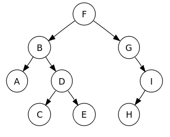
Trees can be traversed in 3 different orders. As trees are recursive data structures, all 3 traversals are defined recursively. The tree below is used as an example in all 3 cases.
Pre-order
- Visit the root
- Pre order traverse the left subtree
- Pre order traverse the right subtree
Pre-order traversal of the tree gives: F B A D C E G I H
In-order
- In order traverse the left subtree
- Visit the root
- In order traverse the right subtree
In-order traversal of the tree gives: A B C D E F G H I
Post-order
- Post order traverse the left subtree
- Post order traverse the right subtree
- Visit the root
Post-order traversal of the tree gives: A C E D B H I G F
Binary Trees
A binary tree is a special case of a tree:
- Each node has at most two children (either 0, 1 or 2)
- The children of the node are an ordered pair (the left node is less than the right node)
A binary tree will always fulfil the following properties:
Where:
- is the number of nodes in the tree
- is the number of external nodes
- is the number of internal nodes
- is the height/max depth of the tree
Binary Tree ADT
The binary tree ADT is an extension of the normal tree ADT with extra accessor methods.
public interface BinaryTree<E> extends Tree<E>{
Node<E> left(Node<E> n); //returns the left child of n
Node<E> right(Node<E> n); //returns the right child of n
Node<E> sibling(Node<E> n); //returns the sibling of n
}
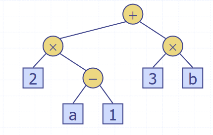
Arithmetic Expression Trees
Binary trees can be used to represent arithmetic expressions, with internal nodes as operators and external nodes as operands. The tree below shows the expression . Traversing the tree in-order will can be used to print the expression infix, and post-order evaluating each node with it's children as the operand will return the value of the expression.
Implementations
- Binary trees can be represented in a linked structure, similar to a linked list
- Node objects are positions in a tree, the same as positions in a positional list
- Each node is represented by an object that stores
- The element
- A pointer to the parent node
- A pointer to the left child node
- A pointer to the right child node
- Alternatively, the tree can be stored in an array
A A[root]is 0- If p is the left child of q,
A[p] = 2 * A[q] + 1 - If p is the right child of q,
A[p] = 2 * A[q] + 2 - In the worst, case the array will have size
Binary Search Trees
- Binary trees can be used to implement a sorted map
- Items are stored in order by their keys
- For a node with key , every key in the left subtree is less than , and every node in the right subtree is greater than
- This allows for support of nearest-neighbour queries, so can fetch the key above or below another key
- Binary search can perform nearest neighbour queries on an ordered map to find a key in time
- A search table is an ordered map implemented using a sorted sequence
- Searches take
- Insertion and removal take time
- Only effective for maps of small size
Methods
Binary trees are recursively defined, so all the methods operating on them are easily defined recursively also.
- Search
- To search for a key
- Compare it with the key at
- If , the value has been found
- If , search the right subtree
- If , search the left subtree
- Insertion
- Search for the key being inserted
- Insert at the leaf reached by the search
- Deletion
- Find the internal node that is follows the key being inserted in an in order traversal (the in order successor)
- Copy key into the in order successor node
- Remove the node copied out of
Performance
- Consider a binary search tree with items and height
- The space used is
- The methods get, put, remove take time
- The height h is in the best case, when the tree is perfectly balanced
- In the worst case, when the tree is basically just a linked list, this decays to
AVL Trees
- AVL trees are balanced binary trees
- For every internal node of the tree, the heights of the subtrees of can differ by at most 1
- The height of an AVL tree storing keys is
- Balance is maintained by rotating nodes every time a new one is inserted/removed
Performance
- The runtime of a single rotation is
- The tree is assured to always have , so the runtime of all methods is
- This makes AVL trees an efficient implementation of binary trees, as their performance does not decay as the tree becomes unbalanced
Priority Queues
A priority queue is an implementation of a queue where each item stored has a priority. The items with the highest priority are moved to the front of the queue to leave first. A priority queue takes a key along with a value, where the key is used as the priority of the item.
Priority Queue ADT
public interface PriorityQueue<K,V>{
int size();
boolean isEmpty();
void insert(K key, V value); //inserts a value into the queue with key as its priority
V removeMin(); //removes the entry with the lowest key (at the front of the queue)
V min(); //returns but not removes the smallest key entry (peek)
}
Entry Objects
- To store a key-value pair, a tuple/pair-like object is needed
- An
Entry<K,V>object is used to store each queue itemKeyis what is used to defined the priority of the item in the queueValueis the queue item
- This pattern is similar to what is used in maps
public class Entry<K,V>{
private K key;
private V value;
public Entry(K key, V value){
this.key = key;
this.value = value;
}
public K getKey(){
return key;
}
public V getValue(){
return value;
}
}
Total Order Relations
- Keys may be arbitrary values, so they must have some order defined on them
- Two entries may also have the same key
- A total order relation is a mathematical concept which formalises ordering on a set of objects where any 2 are comparable.
- A total ordering satisfies the following properties
- or
- Comparability property
- If , then
- Transitive property
- If and , then
- Antisymmetric property
-
- Reflexive property
- or
Comparators
- A comparator encapsulates the action of comparing two objects with a total order declared on them
- A priority queue uses a comparator object given to it to compare two keys to decide their priority
public class Comparator<E>{
public int compare(E a, E b){
if(a < b)
return -1;
if(a > b)
return 1;
return 0;
}
}
Implementations
Unsorted List-Based Implementation
A simple implementation of a priority queue can use an unsorted list
insert()just appends theEntry(key,value)to the list- time
removeMin()andmin()linear search the list to find the smallest key (one with highest priority) to return- Linear search takes time
Sorted List-Based Implementation
To improve the speed of removing items, a sorted list can instead be used. These two implementations have a tradeoff between which operations are faster, so the best one for the application is usually chosen.
insert()finds the correct place to insert theEntry(key,value)in the list to maintain the ordering- Has to find place to insert, takes time
- As the list is maintained in order, the entry with the lowest key is always at the front, meaning
removeMin()andmin()just pop from the front- Takes time
Sorting Using a Priority Queue
The idea of using a priority queue for sorting is that all the elements are inserted into the queue, then removed one at a time such that they are in order
- Selection sort uses an unsorted queue
- Inserting items in each time takes time
- Removing the elements in order
- Overall time
- Insertion sort uses a sorted queue
- Runtimes are the opposite to unsorted
- Adding elements takes time
- Removing elements in each time takes time
- Overall runtime of again
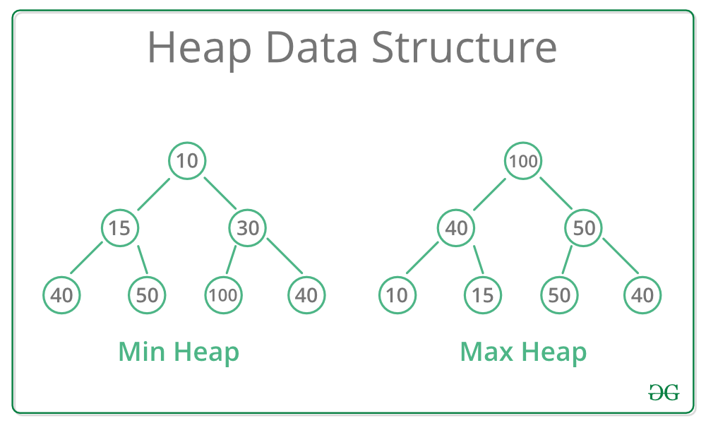
Heaps
- A heap is a tree-based data structure where the tree is a complete binary tree
- Two kinds of heaps, min-heaps and max-heaps
- For a min-heap, the heap order specifies that for every internal node other than the root,
- In other words, the root of the tree/subtree must be the smallest node
- This property is inverted for max heaps
- Complete binary tree means that every level of the tree, except possibly the last, is filled, and all nodes are as far left as possible.
- More formally, for a heap of height , for there are nodes of depth
- At depth , the internal nodes are to the left of the external nodes
- The last node of a heap is the rightmost node of maximum depth
- Unlike binary search trees, heaps can contain duplicates
- Heaps are also unordered data structures
- Heaps can be used to implement priority queues
- An
Entry(Key,Value)is stored at each node
- An
Insertion
- To insert a node
zinto a heap, you insert the node after the last node, makingzthe new last node- The last node of a heap is the rightmost node of max depth
- The heap property is then restored using the upheap algorithm
- The just inserted node is filtered up the heap to restore the ordering
- Moving up the branches starting from the
z- While
parent(z) > (z)- Swap
zandparent(z)
- Swap
- While
- Since a heap has height , this runs in time
Removal
- To remove a node
zfrom the heap, replace the root node with the last nodew - Remove the last node
w - Restore the heap order using downheap
- Filter the replacement node back down the tree
- While
wis greater than either of its children- Swap
wwith the smallest of its children
- Swap
- While
- Also runs in time
Heap Sort
For a sequence S of n elements with a total order relation on them, they can be ordered using a heap.
- Insert all the elements into the heap
- Remove them all from the heap again, they should come out in order
- calls of insert take time
- calls to remove take time
- Overall runtime is
- Much faster than quadratic sorting algorithms such as insertion and selection sort
Array-based Implementation
For a heap with n elements, the element at position p is stored at cell f(p) such that
- If
pis the root,f(p) = 0 - If
pis the left childq,f(p) = 2*f(q)+1 - If
pis the right childq,f(p) = 2*f(q)+2
Insert corresponds to inserting at the first free cell, and remove corresponds to removing from cell 0
- A heap with
nkeys has length
Skip Lists
- When implementing sets, the idea is to be able to test for membership and update elements efficiently
- A sorted array or list is easy to search, but difficult to maintain in order
- Skip lists consists of multiple lists/sets
- The skip list
- contains all the elements, plus
- is a random subset of , for
- Each element of appears in with probability 0.5
- contains only

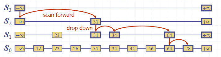
Search
To search for an element in the list:
- Start in the first position of the top list
- At the current position , compare with the next element in the current list
- If , return
- If , move to the next element in the list
- "Scan forward"
- If , drop down to the element below
- "Drop down"
- If the end of the list () is reached, the element does not exist
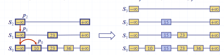
Insertion
To insert an element into the list:
- Repeatedly toss a fair coin until tails comes up
- is the number of times the coin came up heads
- If , add to the skip list new lists
- Each containing only the two end keys
- Search for and find the positions of the items with the largest element in each list
- Same as the search algorithm
- For , insert k into list after position
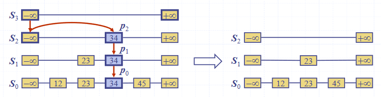
Deletion
To remove an entry from a skip list:
- Search for in the skip list and find the positions of the items containing
- Remove those positions from the lists
- Remove a list if neccessary
Implementation
A skip list can be implemented using quad-nodes, where each node stores
- It's item/element
- A pointer to the node above
- A pointer to the node below
- A pointer to the next node
- A pointer to the previous node
Performance
- The space used by a skip list depends on the random number on each invocation of the insertion algorithm
- On average, the expected space usage of a skip list with items is
- The run time of the insertion is affected by the height of the skip list
- A skip list with items has average height
- The search time in a skip list is proportional to the number of steps taken
- The drop-down steps are bounded by the height of the list
- The scan-forward steps are bounded by the length of the list
- Both are
- Insertion and deletion are also both
Graphs
A graph is a collection of edges and vertices, a pair , where
- is a set of nodes, called vertices
- is a collection of pairs of vertices, called edges
- Vertices and edges are positions and store elements
Examples of graphs include routes between locations, users of a social network and their friendships, and the internet.
There are a number of different types of edge in a graph, depending upon what the edge represents:
- Directed edge
- Ordered pair of vertices
- First vertex is the origin
- Second vertex is the destination
- For example, a journey between two points
- Undirected edge
- Unordered pair of vertices
- In a directed graph, all edges are directed
- In an undirected graph, all edged are undirected
Graph Terminology
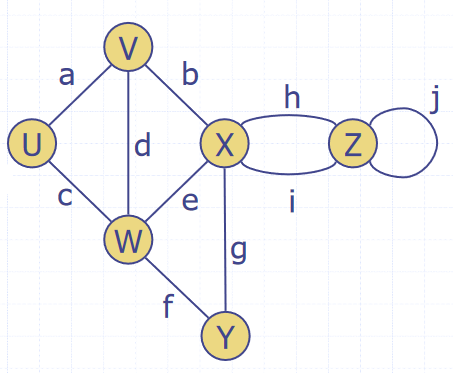
- Adjacent vertices
- Two vertices and are adjacent (ie connected by an edge)
- Edges incident on a vertex
- The edges connect to a vertex
- , , and are incident on
- End vertices or endpoints of an edge
- The vertices connected to an edge
- and are endpoints of
- The degree of a vertex
- The number of edges connected to it
- has degree 5
- Parallel edges
- Edges that make the same connection
- and are parallel
- Self-loop
- An edge that has the same vertex at both ends
- is a self-loop
- Path
- A sequence of alternating vertices and edges
- Begins and ends with a vertex
- Each edge is preceded and followed by its endpoints
- is a simple path
- Cycle
- A circular sequence of alternating vertices and edges
- A circular path
- A simple cycle is one where all edges and vertices are distinct
- A non-simple cycle contains an edge or vertex more than once
- A graph without cycles (acyclic) is a tree
- A circular sequence of alternating vertices and edges
- Length
- The number of edges in a path
- The number of edges in a cycle
Graph Properties
Notation:
- is the number of vertices
- is the number of edges
- is the degree of vertex
The sum of the degrees of the vertices of a graph is always an even number. Each edge is counted twice, as it connects to two vertices, so . For example, the graph shown has and .
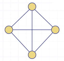
In an undirected graph with no self loops and no multiple edges, . Each vertex has degree at most and . For the graph shown,
The Graph ADT
A graph is a collection of vertices and edges, which are modelled as a combination of 3 data types: Vertex, Edge and Graph.
- A
Vertexis just a box object storing an element provided by the user - An
Edgealso stores an associated value which can be retrieved
public interface Graph{
int numVertices();
Collection vertices(); //returns all the graph's vertices
int numEdges();
Collection<Edge> edges(); //returns all the graph's edges
Edge getEdge(u,v); //returns the edge between u and v, if on exists
// for an undirected graph getEdge(u,v) == getEdge(v,u)
Pair<Vertex, Vertex> endVertices(e); //returns the endpoint vertices of edge e
Vertex oppsite(v,e); //returns the vertex adjacent to v along edge e
int outDegree(v); //returns the number of edges going out of v
int inDegree(v); //returns the number of edges coming into v
//for an undirected graph, inDegree(v) == outDegree(v)
Collection<Vertex> outgoingEdges(v); //returns all edges that point out of vertex v
Collection<Vertex> incomingEdges(v); //returns all edges that point into vertex v
//for an undirected graph, incomingEdges(v) == outgoingEdges(v)
Vertex insertVertex(x); //creates and returns a new vertex storing element x
Edge insertEdge(u,v,x); //creates and returns a new edge from vertices u to v, storing element x in the edge
void removeVertex(v); //removes vertex v and all incident edges from the graph
void removeEdge(e); //removes edge e from the graph
}
Representations
There are many different ways to represent a graph in memory.
Edge List
An edge list is just a list of edges, where each edge knows which two vertices it points to.
- The
Edgeobject stores- It's element
- It's origin
Vertex - It's destination
Vertex
- The edge list stores a sequence of
Edgeobjects
Adjacency List
In an adjacency list, each vertex stores an array of the vertices adjacent to it.
- The
Vertexobject stores- It's element
- A collection/array of all it's incident edges
- The adjacency list stores all
VertexObjects
Adjacency Matrix
An adjacency matrix is an matrix, where is the number of vertices in the graph. It acts as a lookup table, where each cell corresponds to an edge between two vertices.
- If there is an edge between two vertices and , the matrix cell will contain the edge.
- Undirected graphs are symmetrical along the leading diagonal
Subgraphs
- A subgraph of a graph is a graph such that:
- The vertices of are a subset of the vertices of
- The edges of are a subset of the edges of
- A spanning subgraph of is a subgraph that contains all the vertices of
- A graph is connected if there is a path between every pair of vertices
- A tree is an undirected graph such that
- is connected
- has no cycles
- A forest is an undirected graph without cycles
- The connected components of a forest are trees
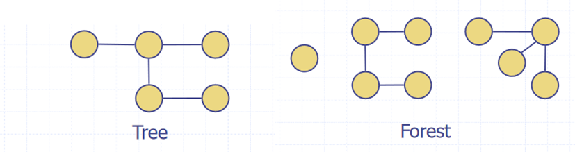
- A spanning tree of a connected graph is a spanning subgraph that has all vertices covered with a minimum possible number of edges
- A spanning tree is not unique unless the graph is a tree
- Multiple spanning trees exist
- Spanning trees have applications in the design of communication networks
- A spanning forest of a graph is a spanning subgraph that is a forest
- A spanning tree is not unique unless the graph is a tree
Depth First Search
DFS is a general technique for traversing a graph. A DFS traversal of a graph will:
- Visit all vertices and edges of
- Determine whether is connected
- Compute the spanning components of
- Compute the spanning forest of
DFS on a graph with vertices and edges takes time. The algorithm is:
- For a graph and a vertex of
- Mark vertex as visited
- For each of 's outgoing edges
- If has not been visited then
- Record as the discovery edge for vertex
- Recursively call DFS with on
- If has not been visited then
DFS(G,V) visits all vertices and edges in the connected component of v, and the discovery edges labelled by DFS(G,V) form a spanning tree of the connected component of v.
DFS can also be extended to path finding, to find a path between two given vertices and . A stack is used to keep track of the path, and the final state of the stack is the path between the two vertices. As soon as the destination vertex is encountered, the contents of the stack is returned.
DFS can be used for cycle detection too. A stack is used to keep track of the path between the start vertex and the current vertex. As soon as a back edge (an edge we have already been down in the opposite direction) is encountered, we return the cycle as the portion of the stack from the top to the vertex .
To perform DFS on every connected component of a graph, we can loop over every vertex, doing a new DFS from each unvisited one. This will detect all vertices in graphs with multiple connected components.
Breadth First Search
BFS is another algorithm for graph traversal, similar to DFS. It also requires time. The difference between the two is that BFS uses a stack while DFS uses a queue. The algorithm is as follows:
- Mark all vertices and edges as unexplored
- Create a new queue
- Add the starting vertex to the queue
- Mark as visited
- While the queue is not empty
- Pop a vertex from the queue
- For all neighbouts of
- If is not visited
- Push into the queue
- Mark as visited
- If is not visited
For a connected component of graph containing :
- BFS visits all vertices and edges of
- The discovery edges labelled by
BFS(G,s)form a spanning tree of - The path of the spanning tree formed by the BFS is the shortest path between the two vertices
BFS can be specialised to solve the following problems in time:
- Compute the connected components of a graph
- Compute a spanning forest of a graph
- Find a simple cycle in G
- Find the shortest path between two vertices
- DFS cannot do this, this property is unique to BFS
Directed Graphs
A digraph (short for directed graph) is a graph whose edges are all directed.
- Each edge goes in only one direction
- Edge goes from a to b but not from b to a
- If the graph is simple and has vertices and edges,
- DFS and BFS can be specialised to traversing directed edges
- A directed DFS starting at a vertex determines the vertices reachable from
- One vertex is reachable from another if there is a directed path to it
Strong Connectivity
A digraph is said to be strongly connected if each vertex can reach all other vertices. This property can be identified in time with the following algorithm:
- Pick a vertex in the graph
- Perform a DFS starting from
- If theres a vertex not visited, return false
- Let be with all the edge directions reversed
- Perform a DFS starting from in
- If theres a vertex not visited, return false
- Else, return True
Transitive Closure
Given a digraph , the transitive closure of is the digraph such that:
- has the same vertices as
- If has a directed path from to , then G* also has a directed *edge* from to
- In , every pair of vertices with a path between them in is now adjacent
- The transitive closure provides reachability information about a digraph

The transitive closure can be computed by doing a DFS starting at each vertex. However, this takes time. Alternatively, there is the Floyd-Warshall algorithm:
- For the graph , number the vertices
- Compute the graphs
- has directed edge if has a directed path from to with intermediate vertices
- Digraph is computed from
- Add if edges and appear in
In pseudocode:
for k=1 to n
Gk = Gk_1
for i=1 to n (i != k)
for j=1 to n (j != i, j!=k)
if G_(k-1).areAdjacent(vi,vk) && G_(k-1).areAdjacent(vk,vj)
if !G_(k-1).areAdjacent(vi,vj)
G_k.insertDirectedEdge(vi,vj,k)
return G_n
This algorithm takes time. Basically, at each iteration a new vertex is introduced, and each vertex is checked to see if a path exists through the newly added vertex. If it does, a directed edge is inserted to transitively close the graph.
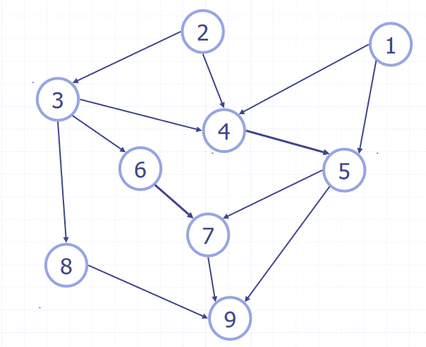
Topological Ordering
- A Directed Acyclic Graph (DAG) is digraph that has no directed cycles
- A topological ordering of a digraph is a numbering of the vertices such that for every edge ,
- The vertex it points to is always greater than it
- A digraph can have a topological ordering if and only if it is a DAG
A topological ordering can be calculated using a DFS:
public static void topDFS(Graph G, Vertex v){
v.visited = true
for(Edge e: v.edges){
w = opposite(v,e)
if(w.visited = false)
topDFS(G,w)
else{
v.label = n
n = n-1
}
}
}
The first node encountered in the DFS is assigned , the one after that , and so on until all nodes are labelled.
CS132
Note that specifics details of architectures such as the 68k, its specific instruction sets, or the PATP are not examinable. They are included just to serve as examples.
The 68008 datasheet can be found here, as a useful resource.
Digital Logic
Digital logic is about reasoning with systems with two states: on and off (0 and 1 (binary)).
Basic Logic Functions
Some basic logic functions, along with their truth tables.
NOT
| A | f |
|---|---|
| 0 | 1 |
| 1 | 0 |
AND
| A | B | f |
|---|---|---|
| 0 | 0 | 0 |
| 0 | 1 | 0 |
| 1 | 0 | 0 |
| 1 | 1 | 1 |
OR
| A | B | f |
|---|---|---|
| 0 | 0 | 0 |
| 0 | 1 | 1 |
| 1 | 0 | 1 |
| 1 | 1 | 1 |
XOR
| A | B | f |
|---|---|---|
| 0 | 0 | 0 |
| 0 | 1 | 1 |
| 1 | 0 | 1 |
| 1 | 1 | 0 |
NAND
| A | B | f |
|---|---|---|
| 0 | 0 | 1 |
| 0 | 1 | 1 |
| 1 | 0 | 1 |
| 1 | 1 | 0 |
NOR
| A | B | f |
|---|---|---|
| 0 | 0 | 1 |
| 0 | 1 | 0 |
| 1 | 0 | 0 |
| 1 | 1 | 0 |
X-NOR
| A | B | f |
|---|---|---|
| 0 | 0 | 1 |
| 0 | 1 | 0 |
| 1 | 0 | 0 |
| 1 | 1 | 1 |
Logic Gates
Logic gates represent logic functions in a circuit. Each logic gate below represents one of the functions shown above.
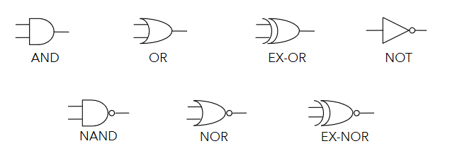
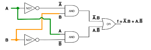
Logic Circuits
Logic circuits can be built from logic gates, where outputs are logical functions of their inputs. Simple functions can be used to build up more complex ones. For example, the circuit below implements the XOR function.
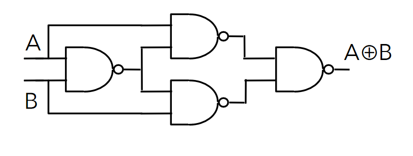
Another example, using only NAND gates to build XOR. NAND (or NOR) gates can be used to construct any logic function.
Truth tables can be constructed for logic circuits by considering intermediate signals. The circuit below has 3 inputs and considers 3 intermediate signals to construct a truth table.
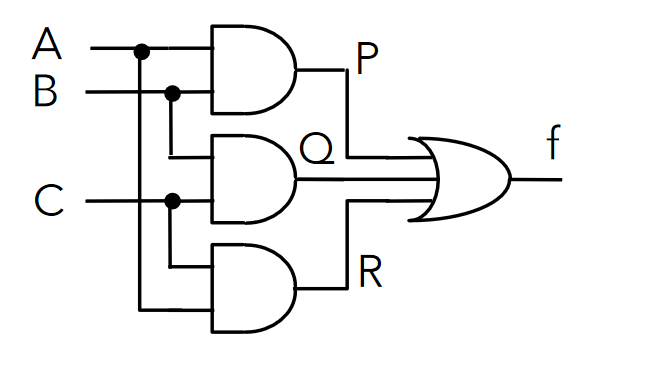
| A | B | C | P | Q | R | f |
|---|---|---|---|---|---|---|
| 0 | 0 | 0 | 0 | 0 | 0 | 0 |
| 0 | 0 | 1 | 0 | 0 | 0 | 0 |
| 0 | 1 | 0 | 0 | 0 | 0 | 0 |
| 0 | 1 | 1 | 0 | 1 | 0 | 1 |
| 1 | 0 | 0 | 0 | 0 | 0 | 0 |
| 1 | 0 | 1 | 0 | 0 | 1 | 1 |
| 1 | 1 | 0 | 1 | 0 | 0 | 1 |
| 1 | 1 | 1 | 1 | 1 | 1 | 1 |
Truth tables of circuits are important as they enumerate all possible outputs, and help to reason about logic circuits and functions.
Boolean Algebra
- Logic expressions, like normal algebraic ones, can be simplified to reduce complexity
- This reduces the number of gates required for their implementation
- The less gates, the more efficient the circuit is
- More gates is also more expensive
- Sometimes, only specific gates are available too and equivalent expressions must be found that use only the available gates
- Two main ways to simplify expressions
- Boolean algebra
- Karnaugh maps
- The truth table for the expression before and after simplifying must be identical, or you've made a mistake
Expressions from Truth Tables
A sum of products form of a function can be obtained from it's truth table directly.
| A | B | C | f |
|---|---|---|---|
| 0 | 0 | 0 | 1 |
| 0 | 0 | 1 | 1 |
| 0 | 1 | 0 | 0 |
| 0 | 1 | 1 | 0 |
| 1 | 0 | 0 | 1 |
| 1 | 0 | 1 | 0 |
| 1 | 1 | 0 | 1 |
| 1 | 1 | 1 | 1 |
Taking only the rows that have an output of 1:
- The first row of the table:
- The second row:
- Fifth:
- Seventh:
- Eight:
Summing the products yields:
Boolean Algebra Laws
There are several laws of boolean algebra which can be used to simplify logic expressions:
| Name | AND form | OR form |
|---|---|---|
| Identity Law | ||
| Null Law | ||
| Idempotent Law | ||
| Inverse Law | ||
| Commutative Law | ||
| Associative Law | ||
| Distributive Law | ||
| Absorption Law | ||
| De Morgan's Law |
- Can go from AND to OR form (and vice versa) by swapping AND for OR, and 0 for 1
Most are fairly intuitive, but some less so. The important ones to remember are:
De Morgan's Laws
De Morgan's Laws are very important and useful ones, as they allow to easily go from AND to OR. In simple terms:
- Break the negation bar
- Swap the operator
Example 1
When doing questions, all working steps should be annotated.
Example 2
Karnaugh Maps
- Karnaugh Maps (k-maps) are sort of like a 2D- truth table
- Expressions can be seen from the location of 1s in the map
| A | B | f |
|---|---|---|
| 0 | 0 | a |
| 0 | 1 | b |
| 1 | 0 | d |
| 1 | 1 | c |
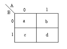
- Functions of 3 variables can used a 4x2 or 2x4 map (4 variables use a 4x4 map)
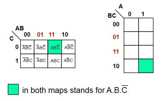
- Adjacent squares in a k-map differ by exactly 1 variable
- This makes the map gray coded
- Adjacency also wraps around
The function is shown in the map below.
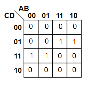
Grouping
- Karnaugh maps contain groups, which are rectangular clusters of 1s -
- To simplify a logic expression from a k-map, identify groups from it, making them as large and as few as possible
- The number of elements in the group must be a power of 2
- Each group can be described by a singular expression
- The variables in the group are the ones that are constant within the group (ie, define that group)
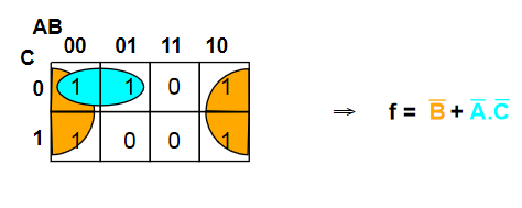
Sometimes, groups overlap which allow for more than one expression
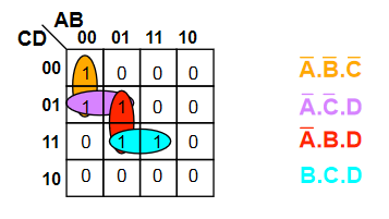
The function for the map is therefore either or (both are equivalent)
Sometimes it is not possible to minimise an expression. the map below shows an XOR function
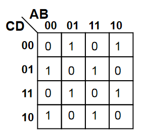
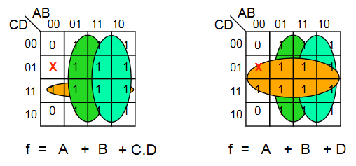
Don't Care Conditions
Sometimes, a certain combination of inputs can't happen, or we dont care about the output if it does. An X is used to denote these conditions, which can be assumed as either 1 or 0, whichever is more convenient.
Combinatorial Logic Circuits
Some useful circuits can be constructed using logic gates, examples of which are shown below. Combinatorial logic circuits operate as fast as the gates operate, which is theoretically zero time (realistically, there is a nanosecond-level tiny propagation delay).
1-Bit Half Adder
- Performs the addition of 2 bits, outputting the result and a carry bit.
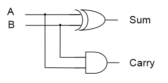
| A | B | Sum | Carry |
|---|---|---|---|
| 0 | 0 | 0 | 0 |
| 0 | 1 | 1 | 0 |
| 1 | 0 | 1 | 0 |
| 1 | 1 | 0 | 1 |
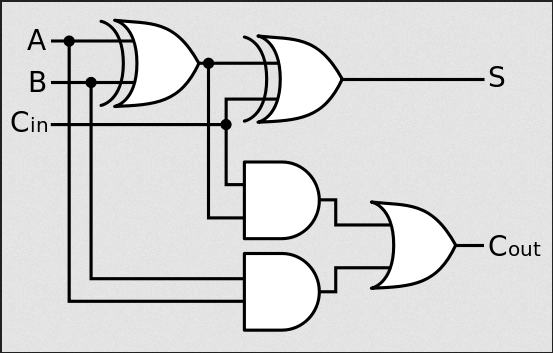
1-Bit Full Adder
- Adds 2 bits plus carry bit, outputting the result and a carry bit.
| Carry in | A | B | Sum | Carry out |
|---|---|---|---|---|
| 0 | 0 | 0 | 0 | 0 |
| 0 | 0 | 1 | 0 | 1 |
| 0 | 1 | 0 | 0 | 1 |
| 0 | 1 | 1 | 1 | 0 |
| 1 | 0 | 0 | 0 | 1 |
| 1 | 0 | 1 | 1 | 0 |
| 1 | 1 | 0 | 1 | 0 |
| 1 | 1 | 1 | 1 | 1 |
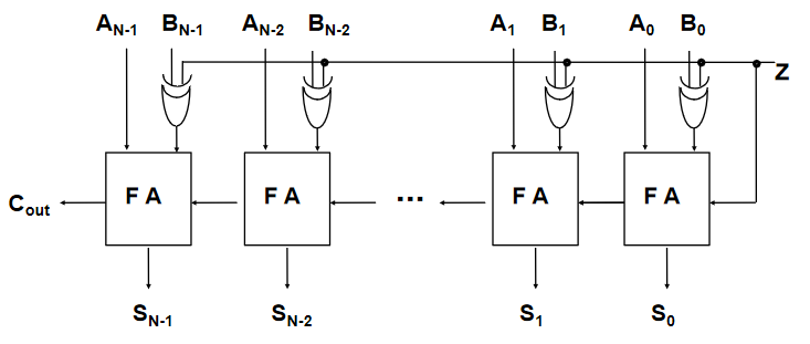
N-Bit Full Adder
- Combination of a number of full adders
- The carry out from the previous adder feeds into the carry in of the next

N-Bit Adder/Subtractor
- To convert an adder to an adder/subtractor, we need a control input such that:
- is calculated using two's complement
- Invert the N bit binary number B by doing
- Add 1 (make the starting carry in a 1)
Encoders & Decoders
- A decoder has binary input pins, and one output pin per possible input state
- eg 2 inputs has 4 unique states so has 4 outputs
- 3 inputs has 8 outputs
- Often used for addressing memory
- The decoder shown below is active low
- Active low means that 0 = active, and 1 = inactive
- Converse to what would usually be expected
- Active low pins sometimes labelled with a bar, ie
- Active low means that 0 = active, and 1 = inactive
- It is important to be aware of this, as ins and outs must comform to the same standard

| 0 | 0 | 0 | 1 | 1 | 1 |
| 0 | 1 | 1 | 0 | 1 | 1 |
| 1 | 0 | 1 | 1 | 0 | 1 |
| 1 | 1 | 1 | 1 | 1 | 0 |
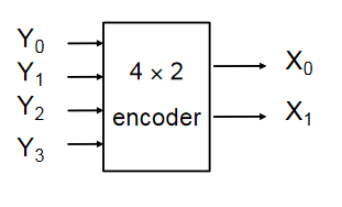
- Encoders are the opposite of decoders, encoding a set of inputs into outputs
- Multiple input pins, only one should be active at a time
- Active low encoder shown below
| 0 | 1 | 1 | 1 | 0 | 0 |
| 1 | 0 | 1 | 1 | 0 | 1 |
| 1 | 1 | 0 | 1 | 1 | 0 |
| 1 | 1 | 1 | 0 | 1 | 1 |
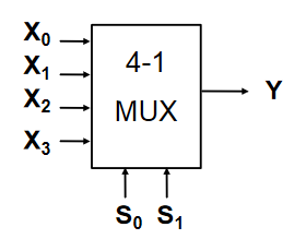
Multiplexers & De-Multiplexers
Multiplexers have multiple inputs, and then selector inputs which choose which of the inputs to put on the output.
| Y | ||
|---|---|---|
| 0 | 0 | |
| 0 | 1 | |
| 1 | 0 | |
| 1 | 1 |
De-Multiplexers are the reverse of multiplexers, taking one input and selector inputs choosing which output it appears on. The one shown below is active low
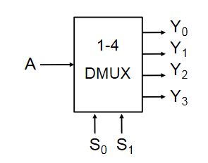
| 0 | 0 | A | 1 | 1 | 1 |
| 0 | 1 | 1 | A | 1 | 1 |
| 1 | 0 | 1 | 1 | A | 1 |
| 1 | 1 | 1 | 1 | 1 | A |
Multiplexers and De-Multiplexers are useful in many applications:
- Source selection control
- Share one communication line between multiple senders/receivers
- Parallel to serial conversion
- Parallel input on X, clock signal on S, serial output on Y
Sequential Logic Circuits
A logic circuit whose outputs are logical functions of its inputs and it's current state
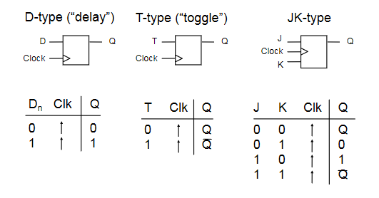
Flip-Flops
Flip-flops are the basic elements of sequential logic circuits. They consist of two nand gates whose outputs are fed back to the inputs to create a bi-stable circuit, meaning it's output is only stable in two states.
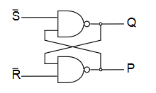
- and are active low set and reset inputs
- is set high when and
- is reset (to zero) when and
- If then does not change
- If both and are zero, this is a hazard condition and the output is invalid
| Q | P | ||
|---|---|---|---|
| 0 | 0 | X | X |
| 0 | 1 | 1 | 0 |
| 1 | 0 | 0 | 1 |
| 1 | 1 | X | X |
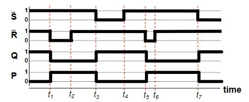
The timing diagram shows the operation of the flip flop
D-Type Latch
A D-type latch is a modified flip-flop circuit that is essentially a 1-bit memory cell.
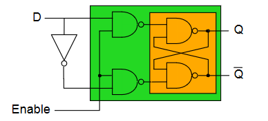
- Output can only change when the enable line is high
- when enabled, otherwise does not change ()
- When enabled, data on goes to
| Enable | |||
|---|---|---|---|
| 0 | 0 | ||
| 0 | 1 | ||
| 1 | 0 | 0 | 1 |
| 1 | 1 | 1 | 0 |
Clocked Flip-Flop
There are other types of clocked flip-flop whose output only changes on the rising edge of the clock input.
- means rising edge responding
N-bit Register
- A multi-bit memory circuit built up from d-type latches
- The number on is stored in the registers when the clock rises
- The stored number appears on the outputs
- cannot change unless the circuit is clocked
- Parallel input, parallel output
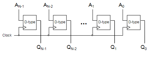
N-bit Shift Register
- A register that stores and shifts bits taking one bit input at a time
- Serial input, parallel output
- When a clock transition occurs, each bit in the register will be shifted one place
- Useful for serial to parallel conversion
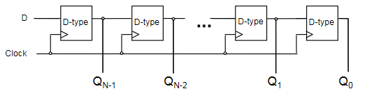
N-bit Counter
- The circles on the clock inputs are inverted on all but the first
- Each flip-flop is triggerd on a high -> low transition of the previous flip-flop
- Creates a counter circuit
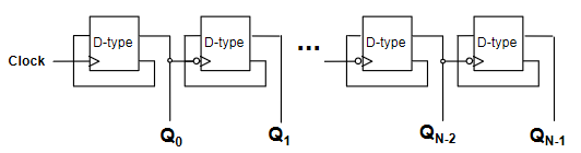
Output is 0000, 1000, 0100, 1100, 0010, etc...
- The first bit swaps every clock
- 2nd bit swaps every other clock
- 3rd bit swaps every fourth clock
- etc...
Three State Logic
- Three state logic introduces a third state to logic - unconnected
- A three-state buffer has an enable pin, which when set high, disconnects the output from the input
- Used to prevent connecting outputs to outputs, as this can cause issues (short circuits)
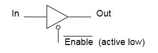
This can be used to allow different sources of data onto a common bus. Consider a 4-bit bus, where 2 4-bit inputs are connected using 3-state buffers. Only one of the buffers should be enabled at any one time.
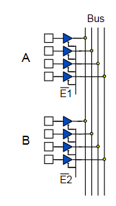
- When , A will be placed on the bus
- When , B will be placed on the bus
Physical Implementations
Logic gates are physical things with physical properties, and these have to be considered when designing with them. Typical voltage values for TTL (Transistor-Transistor Logic):
- 5v - max voltage
- 2.8v - minimum voltage for a logical 1
- 2.8-0.8v - "forbidden region", ie voltages in this region are undefined
- 0.8-0v - voltage range for a logical 0
Propagation Delay
- Logic gates have a propagation delay, the amount of time it takes for the output to reflect the input
- Typically a few nanoseconds or less
- This limits the speed at which logic circuits can operate
- Delay can be reduced by increasing density of gates on an IC
Integrated Circuits
- Elementary logic gates can be obtained in small ICs
- Programmable deviced allow large circuits to be created inside a single chip
- PAL - Programmable Array Logic
- One-time programmamble
- PLA - Programmable Logic Array
- Contains an array of AND and OR gates to implement any logic functions
- FPGA - Field Programmable Gate Array
- Contains millions of configurable gates
- More modern
- PAL - Programmable Array Logic
PLA example
A PLA allows for the implementation of any sum-of-products function, as it has an array of AND gates, then OR gates, with fuses that can be broken to implement a specific function.
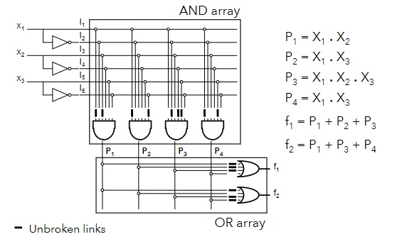
Assembly
Microprocessor Fundamentals
The CPU
- The CPU controls and performs the execution of instructions
- Does this by continuously doing fetch-decode-execute cycle
- Very complex, but two key components
- Control Unit (CU)
- Decodes the instructions and handles logistics
- Arithmetic Logic Unit (ALU)
- Does maths
- Control Unit (CU)
Fetch-Decode-Execute
- Three steps to every cycle
- Fetch instructions from memory
- Decode into operations to be performed
- Execute to change state of CPU
- Takes place over several clock cycles
The components of the CPU that are involved in the cycle:
- ALU
- CU
- Program Counter (PC)
- Tracks the memory address of the next instruction to be executed
- Instruction Register (IR)
- Contains the most recent instruction fetched
- Memory Address Register (MAR)
- Contains address of the memory location to be read/written
- Memory Data/Buffer Register (MDR/MBR)
- Contains data fetched from memory or to be written to memory
The steps of the cycle:
- Fetch
- Instruction fetched from memory location held by PC
- Fetched instruction stored in IR
- PC incremented to point to next instruction
- Decode
- Retrieved instruction decoded
- Establish opcode type
- Execute
- CU signals the necessary CPU components
- May result in changes to data registers, ALU, I/O, etc
The 68008
The 68008 is an example of a CPU. The "programmer's model" is an abstraction that represents the internals of the architecture. The internal registers as shown below are part of the programmer's model.
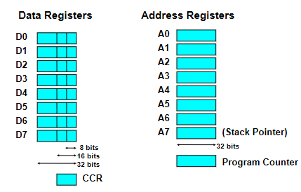
- Internal registers are 32 bits wide
- Internal data buses are 16 bit wide
- 8 bit external data bus
- 20 bit external address bus
- D0-D7 are 32 bit registers used to store frequently used values
- Can be long (32 bits), word (16 bits), or byte (8 bits)
- Status register (CCR) consists of 2 8-bit registers
- Various status bits are set or reset depending upon conditions arising from execution
- A0-A6 are pointer registers
- A7 is system stack pointer to hold subroutine return addresses
- Operations on addresses do not alter status register/ CCR
- Only ALU can incur changes in status
- The stack pointer is a pointer to the next free location in the system stack
- Provides temporary storage of state, return address, registers, etc during subroutine calls and interrupts
The diagram shows the internal architecture of the CPU, and how the internal registers are connected via the buses. Note how and which direction data moves in, as indicated by the arrows on the busses.
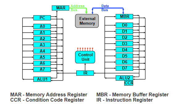
Register Transfer Language
The fetch-decode-execute cycle is best described using Register Transfer Language (RLT), a notation used to show how data moves around the internals of a processor and between registers.
- For example
[MAR] <- [PC]denotes the transfer of the contents of the program counter to the memory address register - Computer's main memory is called Main Store (MS), and the contents of memory location
Nis denoted[MS(N)] - RLT does not account for the pipelining of instructions
- Fetching an instruction in RTL:
| RLT | Meaning |
|---|---|
[MAR] <- [PC] | Move contents of PC to MAR |
[PC] <- [PC] + 1 | Increment PC |
[MBR] <- [MS([MAR])] | Read address from MAR into MBR. |
[IR] <- [MBR] - | Load instruction into I |
CU <- [IR(opcode)] | Decode the instruction |
Assembly Language
- Assembly is the lowest possible form of code
- High level code (for example C) is compiled to assembly code
- Assembly is then assembled into machine code (binary)
- Assembly instructions map 1:1 to processor operations
- Uses mnemonics for instructions, ie
MOVorADD - Languages vary, but format tends to be similar:
LABEL: OPCODE OPERAND(S) | COMMENT
An example program is shown below
ORG $4B0 | this program starts at hex 4B0
move.b #5, D0 | load D0 with number 5
add.b #$A, D0 | add 10 (0x0A) to D0
move.b D0, ANS | move contents of D0 to ANS
ANS: DS.B 1 | leave 1 byte of memory empty and name it ANS
#indicates a literal$means hexadecimal%means binary- A number without a prefix is a memory address
ANSis a symbolic nameORG(Origin) indicates where to load the program in memoryDS(Define Storage) tells the assembler where to put data
The 68008 Instruction Set
- Instructions are commands that tell the processor what to do
- 5 main kinds of instructions
- Logical
- Bitwise operations
AND,LSL(Logical Shift Left)
- Branch
- Cause the processor to jump execution to a labelled address
- Condition is specified by testing state of CCR set by previous instruction
BRA- branch unconditionallyBEQ- branch if equal
- System Control
- Logical
- Instructions are also specified with their data type,
.bfor byte,.wfor word,.lfor longmove.wmoves 2 bytes
Data Movement
- Similar to RTL
move.b D0, D1 | [D1(0:7)] <- [D0(0:7)]
move.w D0, D1 | [D1(0:15)] <- [D0(0:15)]
swap D2 | swap lower and upper words
move.l $F20, D3 | [D3(24:31)] ← [MS($F20)]
| [D3(16:23)] ← [MS($F21)]
| [D3( 8:15)] ← [MS($F22)]
| [D3( 0:7)] ← [MS($F23)]
| copied 8 bytes at a time in big endian order
Arithmetic
- Maths performed on the ALU
- The 68008, like many older processors, has no FPU, so only integer operations are supported
add.l Di, Dj | [Dj] ← [Di] + [Dj]
addx.w Di, Dj | also add in x bit from CCR
sub.b Di, Dj | [Dj] ← [Dj] - [Di]
subx.b Di, Dj | also subtract x bit from CCR
mulu.w Di, Dj | [Dj(0:31)] ← [Di(0:15)] * [Dj(0:15)]
| unsigned multiplication
muls.w Di, Dj | signed multiplication
Logical
- Perform bitwise operations on data
- Also done by ALU
- AND, OR, etc but also shifts and rotates
- Logical shift (
LSL/LSR) adds a 0 when shifting- Bit shifted out goes into C and X
- Arithmetic shift preserves sign bit (
ASL/ASR) - Normal rotate (
ROL/ROR) moves the top of the bit to the bottom bit and also puts the top bit into C and X - Rotate through X (
ROXL/ROXR) rotates the value through the X register
AND.B #$7F, D0 | [D0] <- [D0] . [0x7F]
OR.B D1, D0 | [D0] <- [D0] + [D1]
LSL D0, 2 | [D0] <- [D0] << [2]
Branch
- Cause the processor to move execution to a new pointer (jump/GOTO)
- Instruction tests the state of the CCR bits against certain condition
- Bits set by previous instructions
BRA | branch unconditionally
BCC | branch on carry clear
BEQ | branch on equal
System Control
- Certain instructions used to issue other commands to the microprocessor
Subroutines and Stacks
- Subroutines are useful for frequently used sections of code for obvious reasons
- Can jump and return from subroutines in assembly
JSR <label>- Jump to SubroutineRTS- Return from Subroutine
- When returning, need to know where to return to
- The stack is used as a LIFO data structure to store return addresses
JSRpushes the contents of the PC on the stackRTSpops the return address from the stack to the PC- Can nest subroutine calls and stack will keep track
Addressing Modes
- Addressing modes are how we tell the computer where to find the data it needs
- 5 Kinds in the 68006, and many other processors have equivalents
- Direct
- Immediate
- Absolute
- Address Register Indirect
- 5 variations
- Relative
Direct Addressing
- Probably the simplest
- The address of an operand is specified by either a data or address register
move D3, D2 | [D2] <- [D3]
move D3, A2 | [A2] <- [D3]
Immediate Addressing
- The operand forms part of the instruction (is a literal) and remains a constant
- Note the prefix
#specifying a literal and the prefix specifying the base of the number
move.b #$42, D5 | [D5] <- $42
Absolute Addressing
- Operand specifies the location in memory
- Does not allow for position-independent code: will always access the exact address given
move.l D2, $7FFF0 | [MS(7FFF0)] <- [D2]
Address Register Indirect Addressing
- Uses offsets/increments/indexing to address memory based upon the address registers
- Bad, rarely used
- Not examinable
Relative Addressing
- Specifies an offset relative to the program counter
- Can be used to write position independent code
move 16(PC), D3 | [D3] <- [MS(PC + 16)]
Memory Systems
The Memory Hierarchy
- Memory systems must facilitate the reading and writing of data
- Many factors influence the choice of memory technology
- Frequency of access
- Access time
- Capacity
- Cost
- Memory wants to be low cost, high capacity, and also fast
- As a tradeoff, we organise memory into a hierarchy
- Allows for some high speed, some high capacity
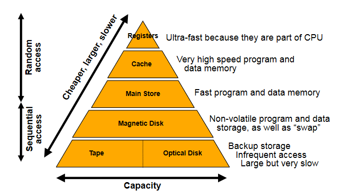
- Data has to be dragged up the hierarchy
- Memory access is somewhat predictable
- Temporal locality - when a location accessed, likely the same location will be accessed again in the near future
- Spatial locality - when a location accessed, likely that nearby locations will be referenced in the near future
- 90% of memory access is within 2Kb of program counter
Semiconductor Memory Types
| Memory Type | Category | Erasure | Write Mechanism | Volatility |
|---|---|---|---|---|
| Random Access Memory (RAM) | Read-Write | Electronically, at byte-level | Electronically written | Volatile |
| Read Only Memory (ROM) | Read only | Not possible | Mask Written | Non-volatile |
| Programmable ROM (PROM) | Read only | Not possible | Electronically written | Non-volatile |
| Erasable PROM (EPROM) | Read (mostly) | UV light at chip level | Electronically written | Non-volatile |
| Electrically Erasable PROM (EEPROM) | Read (mostly) | Electronically, at byte-level | Electronically written | Non-volatile |
| Flash Memory | Read (mostly) | Electronically, at byte-level | Electronically written | Non-volatile |
- Particularly interested in random access
- RAM is most common - implements main store
- nb that all types shown here allow random access, name is slightly misleading
- RAM is also volatile, meaning it is erased when de powered
Cache
- If 90% of memory access is within 2Kb, store those 2Kb somewhere fast
- Cache is small, fast memory right next to CPU
- 10-200 times faster
- If data requested is found in cache, this is a "cache hit" and provides a big speed improvement
- We want things to be in cache
- Cache speed/size is often a bigger bottleneck to performance than clock speed
Moore's Law
- As said by the co-founder of intel, Gordon Moore, the number of transistors on a chip will double roughly every 18 months
- Less true in recent years
- Cost of computer logic and circuitry has fallen dramatically in the last 30 years
- ICs become more densely paced
- CPU clock speed is also increasing at a similar rate
- Memory access speed is improving much more slowly however
Cache Concepts
- Caching read-only data is relatively straightforward
- Don't need to consider the possibility data will change
- Copies everywhere in the memory hierarchy remain consistent
- When caching mutable data, copies can become different between cache/memory
- Two strategies for maintaining parity
- Write through - updates cache and then writes through to update lower levels of hierarchy
- Write back - only update cache, then when memory is replaced copy blocks back from cache
Cache Performance
Cache performance is generally measured by its hit rate. If the processor requests some block of memory and it is already in cache, this is a hit. The hit rate is calculated as
Cache misses can be categorised:
- Compulsory - misses that would occur regardless of cache size, eg the first time a block is accessed, it will not be in cache
- Capacity - misses that occur because cache is not large enough to contain all blocks needed during program execution
- Conflict - misses that occur as a result of the placement strategy for blocks not being fully associative, meaning a block may have to be discarded and retrieved
- Coherency - misses that occur due to cache flushes in multiprocessor systems
Measuring performance solely based upon cache misses is not accurate as it does not take into factor the cost of a cache miss. Average memory access time is measured as hit time + (miss rate miss penalty).
Cache Levels
Cache has multiple levels to provide a tradeoff between speed and size.
- Level 1 cache is the fastest as it is the closest to the cpu, but is typically smallest
- Sometimes has separate instructions/data cache
- Level 2 cache is further but larger
- Level 3 cache is slowest (but still very fast) but much larger (a few megabytes)
- Some CPUs even have a level 4 cache
Different levels of cache exist as part of the memory hierarchy.
Semiconductors
- RAM memory used to implement main store
- Static RAM (SRAM) uses a flip-flop as the storage element for each bit
- Uses a configuration of flip-flops and logic gates
- Hold data as long as power is supplied
- Provide faster read/write than DRAM
- Typically used for cache
- More expensive
- Dynamic RAM (DRAM) uses a capacitor, and the presence to denote a bit
- Typically simpler design
- Can be packed much tighter
- Cheaper to produce
- Capacitor charge decays so needs refreshing by periodically supplying charge
- The interface to main memory is a critical performance bottleneck
Memory Organisation
The basic element of memory is a one-bit cell with two states, capable of being read and written. Cells are built up into larger banks with combinatorial logic circuits to select which cell to read/write. The diagram shows an example of a 16x8 memory IC (16 words of 8 bytes).
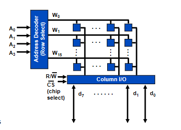
For a 16x8 memory cell:
- 4 address inputs
- 8 data lines
- word size
Consider alternatively a 1Kbit device with 1024 cells
- Organised as a 128x8 array
- 7 address pins
- 8 data pins
- Or, could organise as 1024x1 array
- 10 address pins
- 1 data pins
- Less pins but very poorly organised
- Best to keep memory cells square to make efficient use of space
Error Correction
Errors often occur within computer systems in the transmission of data dude to noise and interference. This is bad. Digital logic already gives a high degree of immunity to noise, but when noise is at a high enough level, this collapses.
Two common ways in which errors can occur:
- Isolated errors
- Occur at random due to noise
- Usually singular incidences
- Burst errors
- Errors usually occur in bursts
- A short period of time over which multiple errors occur
- For example, a 1ms dropout of a connection can error many bits
Majority Voting
- A simple solution to correcting errors
- Just send every bit multiple times (usually 3)
- The one that occurs the most is taken to be the true value
- Slow & expensive
Parity
- Parity adds an extra parity bit to each byte
- Two types of parity system
- Even parity
- The value of the extra bit is chosen to make the total number of 1s an even number
- Odd parity
- The value of the extra bit is chosen to make the total number of 1s an odd number
- Even parity
- 7 bit ascii for
Ais0100 0001- With even parity -
0100 0001 - Odd parity -
1100 0001
- With even parity -
- Can be easily computed in software
- Can also be computed in hardware using a combination of XOR gates
- Usually faster than in software
- Allows for easy error detection without the need to significantly change the model for communication
- Parity bit is computed and added before data is sent, parity is checked when data is received
- Note that if there is more than one error, the parity bit will be correct still and the error won't be detected
- Inadequate for detecting bursts of error
Error Correcting Codes
- ECCs or checksums are values computed from the entire data
- If any of the data changes, the checksum will also change
- The checksum is calculated and broadcast with the data so it can be checked on reception
- Can use row/column parity to compute an checksum
- Calculate parity of each row and of each column
- Diagram shows how parity bits detect an error in the word "Message"
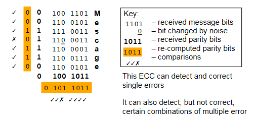
I/O
Memory Mapped I/O
- With memory mapped I/O, the address bus is used to address both memory and I/O devices
- Memory on I/O devices is mapped to values in the main address space
- When a CPU accesses a memory address, the address may be in physical memory (RAM), or the memory of some I/O device
- Advantages
- Very simple
- CPU requires less internal logic
- Can use general purpose memory instructions for I/O
- Disadvantages
- Have to give up some memory
- Less of a concern on 64-bit processors
- Still relevant in smaller 16 bit CPUs
- Have to give up some memory
Polled I/O
- Polling is a technique for synchronising communication between devices.
- Most I/O devices are much slower than the CPU
- Busy-wait polling involves constantly checking the state of the device
- Usually the device replies with nothing
- Can interleave polls with something else useful
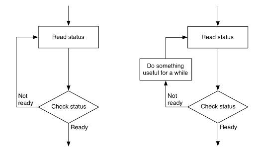
- Advantages
- Still relatively simple
- Disadvantages
- Wastes CPU time and power
- Interleaving can lead to delayed responses from CPU
Synchronisation methods also need some way to transfer the data, so are sometimes used in conjunction with memory-mapped I/O. Methods for synchronising devices and methods for reading/writing data are not directly comparable.
Handshaking
Another form of synchronisation
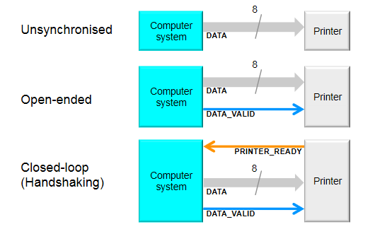
- Computer responds to the printer being ready by placing data on the data bus and signalling
DATA_VALID- Can do this either in hardware or in software
- Timing diagram shows data exchange
- During periods where both signals are at a logical 0, data is exchanged
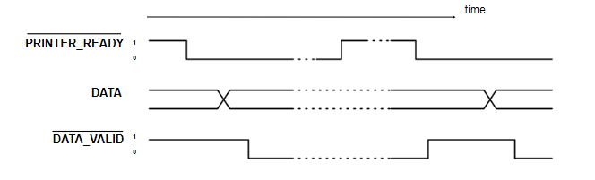
Handshaking Hardware
Handshaking is usually done using an external chip, such as the 6522 VIA (Versatile Interface Adapter)
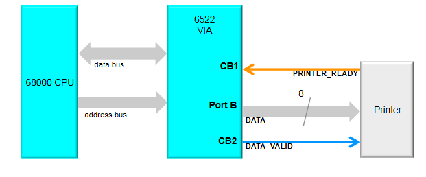
Setting bit values in the PCR (Peripheral Control Register) on the VIA allows to control the function.
- Use PORT B as output
- CB1 control line as
PRINTER_READY - CB2 control line as
DATA_VALID - For CB1 and CB2 control, 8 bit register is set to 1000xxxx
- Last 4 bits not used, don't care
Interrupts
- Asynchronous I/O
- Two kinds of interrupts (in 6502 processor)
- Interrupt Request (IRQ)
- Code can disable response
- Sent with a priority
- If priority lower than that of current task, will be ignored
- Can become non-maskable if ignored for long enough
- Non-Maskable Interrupt (NMI)
- Cannot be disabled, must be serviced
- Interrupt Request (IRQ)
- An interrupt forces the CPU to jump to an Interrupt Service Routine (ISR)
- Switches context, uses stack to store state of registers
- ISRs can be nested
- Interrupts usually generated by some external device
- Hard drive can generate an interrupt when data is ready
- A timer can generate an interrupt repeatedly at a fixed interval
- A printer can generate an interrupt when ready to receive data
- Advantages
- Fast response
- No wasted CPU time
- Disadvantages
- All data transfer still CPU controlled
- More complex hardware/software
Direct Memory Access (DMA)
- The CPU is a bottleneck for I/O
- All techniques shown so far are limited by this bottleneck
- DMA is used where large amounts of data must be transferred quickly
- Control of system busses surrendered from CPU to a DMA Controller (DMAC)
- DMAC is a dedicated device optimised for data transfer
- Can be up to 10x faster than CPU-driven I/O
DMA Operation
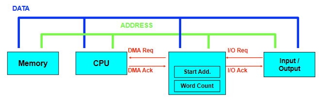
- DMA transfer is requested by I/O
- DMAC passes request to CPU
- CPU initialises DMAC
- Input or Output?
- Start address is put into DMAC address register
- Number of words is put into DMAC count register
- CPU enables DMAC
- DMAC requests use of system busses
- CPU responds with DMAC ack when ready to surrender busses
- DMAC can operate in different modes
- Cycle stealing
- Uses system busses when they're not being used by CPU
- Burst mode
- Requires busses for extended period of time, locks the CPU out for a fixed time, until transfer complete, or until CPU receives interrupt from device of higher priority
- Cycle stealing
DMA Organisation
There are multiple ways a DMA can be incorporated into a system:
- Single bus, detached DMA
- All modules (DMA, I/O devices, memory, CPU) share system bus
- DMA uses programmed I/O to exchanged data between memory and I/O device
- Straightforward, as DMA can just mimic processor
- Inefficient
- Separate I/O bus
- Only one interface to DMA module
- The bus the DMA shares with processor and memory is only used to transfer data to and from memory

Summary
- **Memory-mapped **deviced are accessed in the same way as RAM, at fixed address locations
- Polled I/O is for scheduling input and output, where the CPU repeatedly checks for data
- I/O devices are slow, so handshaking techniques coordinate CPU and device for transfer of data
- Interrupts avoid polled I/O by diverting the CPU to a special I/O routine when necessary
- A DMA controller can be used instead of the CPU to transfer data into and out of memory, faster than the CPU but at additional hardware cost
Microprocessor Architecture
- Computer architecture concerns the structure and properties of a computer system, from the perspective of a software engineer
- Computer organisation concerns the structure and properties of a computer system, from the perspective of a hardware engineer
The PATP
The Pedagogically Advanced Teaching Processor is a very simple microprocessor. The specifics of it are not examinable, but it is used to build an understanding of microprocessor architecture.
Programmer's model
The PATP has 8 instructions. Each instruction is 1 8-bit word, with the first 3 bits as the opcode and last 5 as the operand, if applicable.
| Opcode | Mnemonic | Macro Operation | Description |
|---|---|---|---|
| 000 | CLEAR | [D0] <- 0 | Set D0 to 0 (and set Z) |
| 001 | INC | [D0] <- [D0] + 1 | Increment the value in D0 (and set Z if result is 0) |
| 010 | ADD #v | [D0] <- [D0] + v | Add the literal v to D0 (and set Z if result is 0) |
| 011 | DEC | [D0] <- [D0] - 1 | Decrement the value in D0 (and set Z if result is 0) |
| 100 | JMP loc | [PC] <- loc | Jump unconditionally to address location loc |
| 101 | BNZ loc | If Z is not 0 then [PC] <- loc | Jump to address location loc if Z is not set |
| 110 | LOAD loc | [DO] <- [MS(loc)] | Load the 8 bit value from address location loc to D0 |
| 111 | STORE loc | [MS(loc)] <- [D0] | Write the 8 bit value from D0 to address location loc |
This is not many instructions, but it is technically Turing-complete. The other specs of the PATP are:
- An address space of 32 bytes (the maximum address is
11111) - A single 8-bit data register/accumulator
D0 - A CCR with only 1 bit (
Z, set when an arithmetic operation has a result of zero) - A 5-bit program counter (only 5 bits needed to address whole memory)
Internal Organisation
There are several building blocks that make up the internals of the PATP:
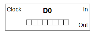
- The data register
D0- An 8 bit register constructed from D-type flip-flops
- Has parallel input and output
- Clocked
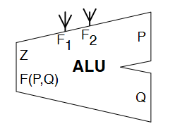
- The ALU
- Built around an 8-bit adder/subtractor
- Has two 8-bit inputs
PandQ - Capable of
- Increment (+1)
- Decrement (-1)
- Addition (+n)
- Two function select inputs
F1andF2which choose the operation to perform- 00: Zero output
- 01: Q + 1
- 10: Q + P
- 11: Q - 1
- An output
F(P, Q)which outputs the result of the operation - A
Zoutput for the CCR
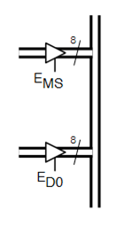
- The main system bus
- Uses 3-state buffers to enable communication
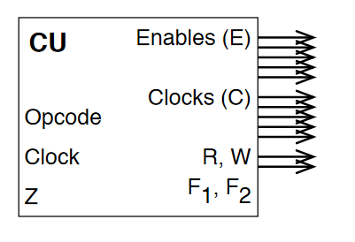
- The control unit
- Controls:
- The busses (enables)
- When registers are clocked
- ALU operation
- Memory acccess
- Responsible for decoding instructions and issuing micro-instructions
- Inputs
- Opcode
- Clock
Zregister
- Outputs
- Enables
- Main store
- Instruction register
IR - Program counter
- Data register
D0 - ALU register
- Clocks
- Memory address register
MAR - Instruction register
IR - Program counter
- Data register
D0 - ALU register
- Memory address register
F1andF2on the ALUR/Wto control bit for main store
- Enables
- Controls:
All the components come together like so:
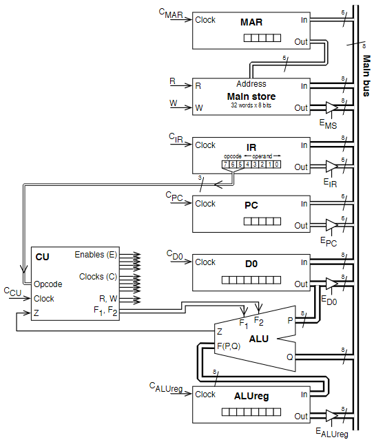
Micro and Macro Instructions
There are several steps internally that are required to execute a single instruction. For example, to execute an INC operation:
- D0 need to be put on the system bus
- CU enables the three-state buffer for D0
[ALU(Q)] <- D0
- The correct ALU function must be selected
F1 = 0,F2 = 1- Signals asserted by CU
[ALU(F)] <- 01
- The output from the ALU must be read into the ALU register
- ALUreg clocked by CU
[ALUreg] <- [ALU]
- D0 reads in the ALU output from the ALU register
- CU enables the three-state buffer for ALUreg
- D0 is clocked by CU
Macro instructions are the assembly instructions issued to the processor (to the CU, specifically), but micro instructions provide a low level overview of how data is moved around between internals of the CPU and what signals are asserted internally. The PATP can execute all instructions in 2 cycles. The table below gives an overview of the micro operations required for each macro instruction, along with the macro operations for fetching from main store.
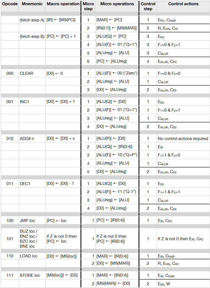
Control Signals
The control unit asserts control signals at each step of execution, and the assertion of these control signals determine how data moves internally. For the PATP:
- Enable signals are level-triggered
- Clock signals are falling edge-triggered
- An output can be enabled onto the main bus and then clocked elsewhere in a single time step
- ALU timings assume that, if values are enabled at P and Q at the start of a cycle, then the ALU register can be clocked on the falling edge of that cycle
- MS timings assume that if MAR is loaded during one cycle, then R, W and EMS can be used in the next cycle
The diagram below shows the timing for a fetch taking 4 cycles, and which components are signalled when. Notice which things happen in the same cycle, and which must happen sequentially.
| cycle | Micro-Op | Control Signals |
|---|---|---|
| 1 | [MAR] <- [PC] | Enable PC, Clock MAR |
| 2 | [IR] <- [MS(MAR)] | Set read for MAR, Enable MS, Clock IR |
| 3 | [ALU(Q)] <- [PC] | Enable PC |
| 3 | [ALU(F) <- 01] | F1 = 0, F2 = 1 |
| 3 | [ALUreg] <- [ALU] | Clock ALUreg |
| 4 | [PC] <- [ALUreg] | Enable ALUreg, Clock PC |
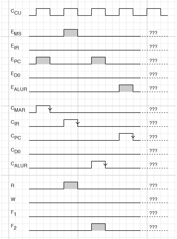
Control Unit Design
The task of the control unit is to coordinate the actions of the CPU, namely the Fetch-Decode-Execute cycle. It generates the fetch control sequence, takes opcode input, and generates the right control sequence based on this. It can be designed to do this in one of two ways:
- Hardwired design (sometimes called "random logic")
- The CU is a combinatorial logic circuit, transforming input directly to output
- Microprogrammed
- Each opcode is turned into a sequence of microinstructions, which form a microprogram
- Microprograms stored in ROM called microprogram memory
Hardwired
- A sequencer is used to sequence the clock cycles
- Has clock input and n outputs
T1 ... Tn - First clock pulse is output from
T1 - Second is output from
T2 - Clock pulse n output from
Tn - Pulse n+1 output from
T1
- Has clock input and n outputs
- This aligns the operation of the circuit with the control steps
- Advantages
- Fast
- Disadvantages
- Complex, difficult to design and test
- Inflexible, cant change design to add new instructions
- Takes a long time to design
- This technique is most commonly used in RISC processors and has been since the 80s
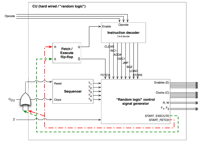
- The control signal generator maps each instruction to outputs
- The sequencer sequences the outputs appropriately
- The flip-flop is used to regulate control rounds
Microprogrammed
- The microprogram memory stores the required control actions for each opcode
- The CU basically acts as a mini CPU within the CPU
- Microaddress is a location within microprogram memory
- MicroPC is the CU's internal program counter
- MicroIR is the CU's internal microinstruction register
- The microPC can be used in different ways depending upon implementation
- Holds the next microaddress
- Holds the microaddress of microroutine for next opcode
- When powered initially holds microaddress 0
- The fetch microprogram
- Each microinstruction sets the CU outputs to the values dictated the instruction
- As the microprogram executes, the CU generates control signals
- After each microinstruction, the microPC is typically incremented, so microinstructions are stepped through in sequence
- After a fetch, the microPC is not incremented, but is set to the output from the opcode decoding circuit (labelled OTOA in the diagram)
- After a normal opcode microprogram, the microPC is set back to 0 (fetch)
- When executing the microprogram for a conditional branch instruction, the microPC value is generated based upon whether the CU's Z input is set
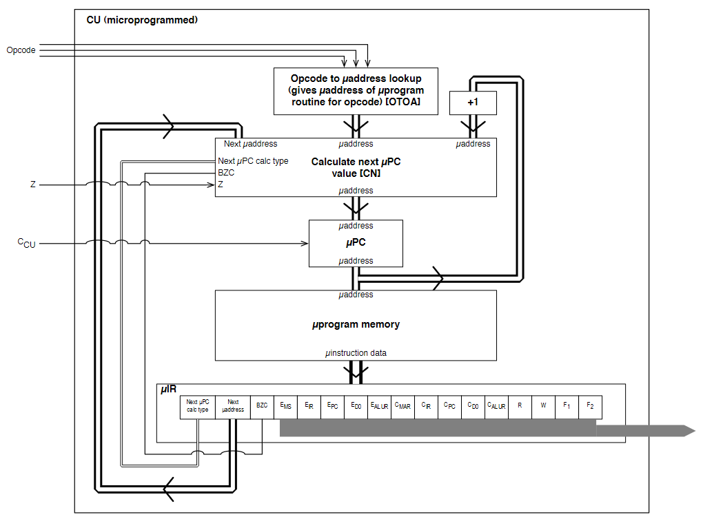
- Advantages
- Easy to design and implement
- Flexible design
- Simple hardware compared to alternative
- Can be reprogrammed for new instructions
- Disadvantages
- Slower than hardwired
- Most commonly used for CISC processors
RISC and CISC
In the late 70s-early 80s, it was shown that certain instructions are used far more than others:
- 45% data movement (move, store, load)
- 29% control flow (branch, call, return)
- 11% arithmetic (add, sub)
The overhead from using a microprogram memory also became more significant as the rest of the processor became faster. This caused a shift towards RISC computing. Right now, ARM is the largest RISC computing platform. Intel serve more for backwards compatibility with a CISC instruction set. In an modern intel processor, simplest instructions are executed by a RISC core, more complex ones are microprogrammed.
- RISC has simple, standard instructions whereas CISC has lots of more complex instructions
- x86 is often criticised as bloated
- RISC allows for simpler, faster, more streamlined design
- RISC instructions aim to be executed in a single cycle
- CISC puts the focus on the hardware doing as much as possible, whereas RISC makes the software do the work
Multicore Systems
- The performance of a processor can be considered as the rate at which it executes instructions: clock speed x IPC (instructions per clock).
- To increase performance, increase clock speed and/or IPC
- An alternative way of increasing performance is parallel execution
- Multithreading separates the instruction stream into threads that can execute in parallel
- A process is an instance of a program running on a computer
- A process has ownership of resources: the program's virtual address space, i/o devices, other data that defines the process
- The process is scheduled by the OS to divide the execution time of the processor between threads
- The processor switches between processes using the stack
CS141
#notacult
Types & Typeclasses
Haskell is a strongly, statically typed programming language, which helps prevent us from writing bad programs.
- Java, C, Rust - strongly typed
- Python, Ruby - dynamically typed
Types have many benefits:
- Describe the value of an expression
- Prevent us from doing silly things
not 7givesType Error
- Good for documentation
- Type errors occur at compile time
GHC checks types and infers the type of expressions for us. Types are discarded after type checking, and are not available at runtime.
Type notation
We say an expression has a type by writing expression :: type, read as "expression has type".
- If we can assign a type to an expression, it is "well typed"
- A type approximates and describes the value of an expression.
42 :: Int
True :: Bool
'c' :: Char
"Cake" :: String
0.5 :: Double
4 + 8 :: Int
2 * 9 + 3 :: Int
True && False :: Bool
"AB" ++ "CD" :: String
even 9 :: Bool
Before writing a definition, it is good practice to write its type.
daysPerWeek :: Int
daysperWeek = 7
Function Types
The types of functions are denoted using arrows ->. The not function is defined as not :: Bool -> Bool, read "not has type bool to bool". It means if you give me a Bool, I will give you back another Bool.
The definition of the not function is shown below.
not :: Bool -> Bool
not True = False
not False = True
not True :: Bool
The last line shows how function application eliminates function types, as by applying a function to a value, one of the types from the function definition is removed as it has already been applied.
The xor function takes two boolean arguments and is defined:
xor :: Bool -> Bool -> Bool
xor False True = True
xor False False = False
xor True True = False
xor True False = True
Applying one argument to a function that takes two is called partial function application, as it partially applies arguments to a function to return another function. This is because all functions in haskell are curried, meaning all functions actually only take one argument, and functions taking more than one argument are constructed from applying multiple functions with one argument.
xor :: Bool -> Bool -> Bool
xor True :: Bool -> Bool -- partially applied function
xor True False :: Bool
Polymorphic Types
What is the type of \x -> x ? Could be:
f :: Int -> Int
f :: Bool -> Bool
f :: Char -> Char
These are all permissible types. To save redifining a function, we can use type variables. Anything with a single lowercase character is a type variable (a in this case).
\x -> x :: a -> a
\x -> x is the identity function, as it returns its argument unchanged. We can also have functions with more than one type variable, to specify that arguments have different types:
const :: a -> b -> a
const x y = x
Tuples
Tuples are a useful data structure
(4, 7) :: (Int, Int)
(4, 7.0) :: (Int, Double)
('a', 9, "Hello") :: (Char, Int, String)
--can nest tuples
((4, 'g'), False) :: ((Int, Char), Bool)
--can also contain functions
(\x -> x, 8.15) :: (a->a, Double)
Functions on pairs. These are all in the standard library
fst :: (a,b) -> a
snd :: (a,b) -> b
swap :: (a,b) -> (b,a)
-- these functions can also be defined by pattern matching
fst (x,y) = x
snd (x,y) = y
swap (x,y) = (y,x)
Type Classes
Type classes are used for restricting polymorphism and overloading functions.
- The
(+)operator probably has type(+) :: Int -> Int -> Int,- This is correct, as this typing is permissible
- What about
1.2 + 3.4?- Will raise an error with this definition of
(+)
- Will raise an error with this definition of
- Can polymorphism help?
(+) :: a -> a -> a- This is stupid
- Allows any types
- Won't work
- A type class constraint is needed
- The actual type is
(+) :: Num a => a -> a -> a- The
Num a =>part is the constraint part - Tells the compiler that
ahas to belong to the typeclassNum
- The
- Type class constraints are used to constrain type variables to only types which support the functions or operators specified by the type class
- Type class names start with an uppercase character
Numis a type class that represents all types which support arithmetic operations
Defining Type Classes
A type class is defined as follows:
class Num a where
(+) :: a -> a -> a
(-) :: a -> a -> a
abs :: a -> a
Numis the name of the type classais the type variable representing it in the method typings- The type class contains method signatures for all functions that members of the type class must implement
The type class contains type definitions, but no implementations for the functions. To implement them, we need to tell the compiler which types implement the type class and how they implement the functions in the type class. The Show typeclass tells the compiler that a type can be converted to a string.
-- typeclass definition
class Show a where
show :: a -> String
-- instance of typeclass for bool type
instance Show Bool where
show True = "True"
show False = "False"
The instance definition tells the compiler that Bool is a member of Show, and how it implements the functions that Show defines.
Prelude Type Classes
Numfor numbersEqfor equality operators==/=Ordfor inequality/comparison operators><=etcShowfor converting things to string- Many More
The REPL makes extensive use of Show to print things. There are no show instances for function types, so you get an error if you try to Show functions. Typing :i in the REPL gets info on a type class. :i Num gives:
class Num a where
(+) :: a -> a -> a
(-) :: a -> a -> a
(*) :: a -> a -> a
negate :: a -> a
abs :: a -> a
signum :: a -> a
fromInteger :: Integer -> a
{-# MINIMAL (+), (*), abs, signum, fromInteger, (negate | (-)) #-}
-- Defined in ‘GHC.Num’
instance Num Word -- Defined in ‘GHC.Num’
instance Num Integer -- Defined in ‘GHC.Num’
instance Num Int -- Defined in ‘GHC.Num’
instance Num Float -- Defined in ‘GHC.Float’
instance Num Double -- Defined in ‘GHC.Float’
Types of Polymorphism
In Java, there are two kinds of polymorphism:
- Parametric polymorphism
- (Generics/Templates)
- A class is generic over certain types
- Can put whatever type you like in there to make a concrete class of that type
- Subtype polymorphism
- Can do
class Duck extends Bird - Can put
Ducks whereverBirds are expected
- Can do
Haskell has two kinds of polymorphism also:
- Parametric polymorphism
- Type variables
id :: a -> a- Can accept any type where
ais
- Ad-hoc polymorphism
- Uses type classes
double :: Num a => a -> adouble x = x * 2
Further Uses of Constraints
An example Show instance for pairs:
instance (Show a, Show b) => Show (a,b) Show where
show (x,y) = "(" ++ show x ++ ", " ++ show y ++ ")"
The (Show a, Show b) => defines a constraint on a and b that they must both be instances of show for them to be used with this instance. The instance is actually defined on the type (a,b).
Can also define that a typeclass has a superclass, meaning that for a type to be an instance of a typeclass, it must be an instance of some other typeclass first. The Ord typeclass has a superclass constraint of the Eq typeclass, meaning something cant be Ord without it first being Eq. This makes sense, as you can't have an ordering without first some notion of equality.
class Eq a => Ord a where
(<) :: a -> a -> Bool
(<=) :: a -> a -> Bool
Default Implementations
Type classes can provide default method implementations. For example, (<=) can be defined using the definition of (<), so a default one can be provided using (==)
class Eq a => Ord a where
(<) :: a -> a -> Bool
(<=) :: a -> a -> Bool
(<=) x y = x < y || x == y
-- or defined infix
x <= y = x < y || x == y
Derivable Type Classes
Writing type class instances can be tedious. Can use the deriving keyword to automatically generate them, which does the same as manually defining type class instances.
data Bool = False | True
deriving Eq
data Module = CS141 | CS118 | CS126
deriving (Eq, Ord, Show)
Certain other typeclasses can be dervied too, by enabling language extensions within GHC. The extension XDeriveFunctor allows for types to include a deriving Functor statement.
Data Types
How do we make our own data types in haskell? Algebraic data types.
Boolis a type- There are two values of type
BoolTrueFalse
data Bool = True | False
A type definition consists of the type name Bool and it's data constructors, or values True | False. A type definition introduces data constructors into scope, which are just functions.
True :: Bool
False :: Bool
We can pattern match on data constructors, and also use them as values. This is true for all types.
not :: Bool -> Bool
not True = False
not False = True
More examples:
data Module = CS141 | CS256 | CS263
data Language = PHP | Java | Haskell | CPP
--for this one, the type name and constructor name are separate names in the namespace
data Unit = Unit
-- this one has no values
data Void
Parametrised Data Constructors
Parameters can be added to a data constructor by adding their types after the constructor's name. The example below defines a type to represent shapes. Remember that data constructors are just functions, and can be partially applied just like other functions.
data Shape = Rect Double Double | Circle Double
Rect :: Double -> Double -> Shape
Circle :: Double -> Shape
-- functions utilising the Shape type
-- constructs a square
square x :: Double -> Shape
square x = Rect x x
-- calculates area of a shape using pattern matching on constructors
area :: Shape -> Double
area (Rect w h) = w * h
area (Circle r) = pi * r * r
isLine :: Shape -> Bool#
isLine (Rect 1 h) = True
isLine (Rect w 1) = True
isLine _ = False
-- examples
area (square 4.0)
=> area (Rect 4.0 4.0)
=> 4.0 * 4.0
=> 16.0
area (Circle 5.0)
=> pi * 5.0 * 5.0
=> pi * 25.0
=> 78.53981...
Parametrised Data Types
The Maybe type is an example of a data type parametrised over some type variable a. It exists within the standard library, defined as data Maybe a = Nothing | Just a. This type is used to show that either there is no result, or some type a.
A function using the Maybe type to perform devision safely, returning Nothing if the divisor is 0, and the result wrapped in a Just if the division can be done.
data Maybe a = Nothing | Just a
safediv :: Int -> Int -> Maybe Int
safediv x 0 = Nothing
safediv x y = Just (x `div y)
-- safediv 8 0 => Nothing
-- safediv 8 4 = Just (8 `div` 4) = Just 2
-- this is included in stdlib for extracting the value using pattern matching
fromMaybe :: a -> Maybe a -> a
fromMaybe x Nothing = x
fromMaybe _ (Just x) = x
Null references were invented in the 1960s ... the guy who invented them called them his "billion dollar mistake". The Maybe type is a good alternative, which makes it clear that a value may be absent. Similar concepts exist in other procedural languages (Swift, Rust)
Recursive Data Types
In Haskell, data types can be defined in terms of themselves. An example definition of the natural numbers is shown below, where a number is either zero, or one plus another number.
data Nat = Zero | Succ Nat
Zero :: Nat
Succ :: Nat -> Nat
one = Succ Zero
two = Succ one
three = Succ two
add :: Nat -> Nat -> Nat
add Zero m = m
add (Succ n) m = Succ (add n m)
mul :: Nat -> Nat -> Nat
mul Zero m = Zero
mul (Succ n) m = add m (mul n m)
Another example defining binary trees in terms of themselves. A binary tree consists of subtrees (smaller binary trees). This type is parametrised over some type variable a also.
Data BinTree a = Leaf a | Node (BinTree a) (BinTree a)
--converts a binary tree to a list
flatten :: BinTree a -> [a]
flatten (Leaf x) = [x]
flatten (Node l r) = flatten l ++ flatten r
-- computes the max depth of the tree
depth :: BinTree a -> Int
depth (Leaf _) = 1
depth (Node l r) = 1 + max (depth l) (depth r)
Type Aliases
Types can be aliased. For example, String has been an alias of [Char] all along.
type String = [Char]
Another example, defining a Predicate type
type Predicate a = a -> Bool
isEven :: Predicate Int
isEven n = n `mod` 2 == 0
isEven' :: (Eq a, Integral a) => Predicate a
isEven' n = n `mod` 2 == 0
Recursion
Recursion is a way of expressing loops with no mutable state, by defining a function in terms of itself. The classic example, the factorial function. Defined mathematically:
In haskell:
factorial :: Int -> Int
factorial 0 = 1
factorial n = n * factorial (n-1)
It can be seen how this function reduced when applied to a value:
factorial 2
=> 2 * factorial (2-1)
=> 2 * factorial 1
=> 2 * 1 * factorial (1-1)
=> 2 * 1 * factorial 0
=> 2 * 1 * 1
=> 2
Another classic example, the fibonacci function:
fib :: Int -> Int
fib 0 = 1
fib 1 = 1
fib n = fib (n-1) + fib (n-1)
In imperative languages, functions push frames onto the call stack every time a function is called. With no mutable state, this is not required so recursion is efficient and can be infinite.
Haskell automatically optimises recursive functions to make execution more efficient:
fac' :: Int -> Int -> Int
fac' 0 m = m
fac' n m = fac' (n-1) (n*m)
This version of the function prevents haskell from building up large expressions:
fac 500
=> fac' 500 1
=> fac' (500-1) (500*1)
=> fac' 499 500
=> fac (499-1) (499 * 500)
=> fac' 498 249500
Notice the pattern for all recursive functions, where there is a recursive case, defining the function in terms of itself, and a base case. Without a base case, the function would recurse infinitely. The cases are usually defined as pattern matches.
Recursion on Lists
Recursion is the natural way to operate on lists in haskell. Defining the product function, which returns the product of all the items in the list:
product :: [Int] -> Int
product [] = 1
product (n:ns) = n * product ns
Here, the base case is the empty list [] and pattern match is used to "de-cons" the head off the list and operate on it (n:ns). The function reduces as follows:
product [1,2,3,4]
=> 1 * product [2,3,4]
=> 1 * 2 * product [3,4]
=> 1 * 2 * 3 * product [4]
=> 1 * 2 * 3 * 4 * product []
=> 1 * 2 * 3 * 4 * 1
=> 24
let and where
let and where clauses can be used to introduct local bindings within a function, which are useful in defining recursive functions. the splitAt function, which splits a list into two at a certain index.
splitAt :: Int -> [a] -> ([a],[a])
splitAt 0 xs = ([],xs)
splitAt n [] = ([],[])
splitAt n (x:xs) = (x:ys, zs)
where (ys,zs) = splitAt (n-1) xs
-- alternatively
splitAt n xs =
let
ys = take n xs
zs = drop n xs
in (ys,zs)
let and where can also define functions locally, as everything in haskell is a function.
Higher Order Functions
Higher order functions are functions which operate on functions.
Associativity of functions
Function expressions associate to the right (one argument is applied at a time)
xor a b = (a || b ) && not (a && b)
-- equivalent to
xor = \a -> \b -> (a || b) && not (a && b)
-- equivalent to
xor = \a -> (\b -> (a || b) && not (a && b))
- All functions in haskell are technically nameless, single-parameter functions
- Currying allows for functions which return other functions
- Functions are expressions
- The body of a function is an expression
- When a function is applied to an argument it reduces to it's body.
Function application associates to the left:
xor True True
=> (xor True) True
=> ((\a -> (\b -> (a || b) && not (a && b))) True) True
=> (\b -> (True || b) && not (True && b)) True
=> (True || True) && not (True && True)
Function types, however, associate to the right:
xor :: Bool -> Bool -> Bool
xor = \a -> \b -> (a || b) && not (a && b)
--equivalent to
xor :: Bool -> (Bool -> Bool)
xor = xor = \a -> (\b -> (a || b) && not (a && b))
The table below shows how functions application and types associate:
| Without Parentheses | With Parentheses |
|---|---|
f x y | (f x) y |
\x -> \y -> ... | \x -> (\y -> ...) |
Int -> Int -> Int | Int -> (Int -> Int) |
Functions as Arguments (map)
Haskell functions can be taken as arguments to other functions. Functions that take/return functions are called higher order functions. An example, increasing every element of a list by one:
incByOne :: [Int] -> [Int]
incByOne xs = [x+1 | x <- xs]
-- or using recursion
incByOne [] = []
incByOne (x:xs) = x+1 : incByOne xs
All this function does is applies the function (+ 1) to every element. This pattern can be generalised using the map function: a function that applies a function given as an argument to every element of a list:
map :: (a -> b) -> [a] -> [b]
map f [] = []
map f (x:xs) = f x : map f xs
Note the type signature of the map function is map :: (a -> b) -> [a] -> [b], meaning the first argument is a function of type (a -> b). Using this to implement incByOne:
incByOne = map (+1)
-- tracing it's evaluation:
incByOne [1,2,3]
=> map (+1) [1,2,3]
=> (1+1) : map (+1) [2,3]
=> (1+1) : (1+2) : map (+1) [3]
=> (1+1) : (1+2) : (1+3) : map (+1) []
=> (1+1) : (1+2) : (1+3) : []
=> [2,3,4]
Effectively, map f [x, y, z] evaluates to [f x, f y, f z]
Sections
Sections are partially applied operators. Operators are functions like any other, and as such can be partially applied, passed as arguments, etc. The addition operator is shown as an example, but the same applies to any binary operator.
(+) :: Num a => a -> a -> a
(+ 4) :: Num a => a -> a
(4 +) :: Num a => a -> a
(+) 4 8 = 4 + 8
(+ 4) 8 = 8 + 4
(4 +) 8 = 4 + 8
Filter
Filter is an example of another higher order function, which given a list, returns a new list which contains only the elements satisfying a given predicate.
filter :: (a -> Bool) -> [a] -> [a]
filter p [] = []
filter p (x:xs)
| p x = x : filter p xs
| otherwise = filter p xs
Some examples:
-- remove all numbers less than or equal to 42
greaterThan42 :: (Int -> Bool) -> [Int] -> [Int]
greaterThan42 xs = filter (>42) xs
-- only keep uppercase letters
uppers :: (Char -> Bool) -> String -> String
uppers xs = filter isUpper xs
Curried vs Uncurried
Tuples can be used to define uncurried functions. A function that takes two arguments can be converted to a function that takes an a tuple of two arguments, and returns a single argument/
uncurriedAdd :: (Int, Int) -> Int
uncurriedAdd (x, y) = x + y
There are higher-order functions, curry and uncurry, which will do this for us:
curry :: ((a,b) -> c) -> a -> b -> c
curry f x y = f (x,y)
uncurry :: (a -> b -> c) -> (a,b) -> c
uncurry f (x,y) = f x y
-- examples
uncurriedAdd :: (Int, Int) -> Int
uncurriedAdd = uncurry (+)
curriedAdd :: Int -> Int -> Int
curriedAdd = curry uncurriedAdd
addPairs :: [Int]
addPairs = map (uncurry (+)) [(1, 2), (3, 4)]
Folds
foldr and foldl "collapse" a list by applying a function f to each element in the list in turn, where the first argument is an accumulated value, and the second is the starting value passed. There are several functions which follow this pattern, all reducing a list to a single value using recursion:
-- and together all bools in the list
and :: [Bool] -> Bool
and [] = True
and (b:bs) = ((&&) b) (and bs)
-- product of everything in the list
product :: Num a => [a] -> a
product [] = 1
product (n:ns) = ((*) n) (product ns)
-- length of list
length :: [a] -> Int
length [] = 0
length (x:xs) = ((+) 1) (length xs)
All of these functions have a similar structure, and can be redefined using foldr:
foldr :: (a -> b -> b) -> b -> [a] -> b
foldr f z [] = z
foldr f z (x:xs) = f x (foldr f z xs)
-- examples
and :: [Bool] -> Bool
and = foldr (&&) True
product :: Num a => [a] -> a
product = foldr (*) 1
length :: [a] -> Int
length = foldr (\x n -> n + 1) 0
In essence, foldr f z [1, 2, 3] is equal to f 1 (f 2 (f 3 z)). foldr folds from right (r) to left, starting by applying the function to the last element of the list first. foldl, however, works in the opposite direction:
foldl :: (b -> a -> b) -> b -> [a] -> b
foldl f z [] = z
foldl f z (x:xs) = foldl f (f z x) xs
foldl f z [1, 2, 3] is equal to f (f (f z 1) 2) 3. For some functions (commutative ones), there is no difference, but often the choice of which to use is important.
Function Composition
In haskell, functions are composed with the (.) operator, a higher order function defined as:
(.) :: (b -> c) -> (a -> b) -> a -> c
(.) f g x = f (g x)
Function composition is used to chain functions, so instead of f (g (h x)), you can write f.g.h x. An example, defining a function count to count the number of occurrences of an element in a list:
count :: Eq a => a => [a] -> Int
count _ [] = 0
count y (x:xs)
| y == x = 1 + count y xs
| otherwise = count y xs
--alternatively, using a fold
count y = foldr (\x l -> if y==x then 1+l else l) 0
-- the stdlib can do this
count y x = length (filter (==y) xs)
count y = length . filter (==y) -- using composition
Lazy Evaluation
Evaluation Strategies
How are programs evaluated? There are a number of strategies for evaluating a program. For example, the expression (4+8) * (15 + 16) can be evaluated in different ways:
(4+8) * (15 + 16)
=> 12 * (15+16)
=> 12 * 31
=> 372
-- or
(4+8) * (15 + 16)
=> (4 + 8) * 31
=> 12 * 31
=> 372
The final value when reducing an expression (it cannot be reduced further) is the normal form, 372 in this case. No matter how the expression is reduced, the normal form is the same. Haskell's type system prevents us from writing anything that cannot reduce to normal form.
A sub-expression (anything partially reduced that can still be reduced further) is called a redex, short for reducible expression. Evaluation strategies only matter when there are multiple redexes, otherwise there is only one route we can take to evaluate an expression.
Strict Evaluation
A programming language is strict if the arguments of the function are evaluated before the function is called.
Evaluating fac 500 using a strict method:
fac :: Int -> Int
fac n = fac' n 1
fac' :: Int -> Int -> Int
fac n m = case n of
0 -> m
_ -> fac' (n-1) (n*m)
fac 500 -- a redex, function application
=> fac' 500 1 -- another redex
=> fac' (500-1) (500*1) -- 3 redexes, two multiplications and function application
=> fac' 499 (500*1) -- two redexes now as 500-1=499 is now in normal form
=> fac' 499 500 -- now only one redex
=> fac' (499-1) (499*500) -- back to 3 redexes
... -- this goes on for a while
Call-by-value means that all function arguments are reduced to their normal forms (values), and then passed as such to the function. The call-by-value strategy is an example of strict evaluation. This is the evaluation strategy used by most programming languages: Java, JS, PHP, C/C++, OCaml, F#, Python, Scala, Swift. Note that some of these are also functional languages.
Haskell, on the other hand, is far superior. It is non-strict: aka lazy.
Call-by-name
A non-strict evaluation strategy by which expressions given to functions as arguments are not reduced before the function call is made.
Expressions are only reduced when their value is needed. Same example as before:
fac 2
=> fac' 2 1 -- still a redex here
=> case 2 of
0 -> 1
_ -> fac' (2-1) (2*1) -- the function call is expanded to its expression
=> fac' (2-1) (2*1) -- left with 3 redexes now
=> case 2-1 of
0 -> 2*1
_ -> fac' ((2-1)-1) ((2-1) * (2*1)) -- a lot of redexes, but we don't need to know the value of any except the one in the case expression. this one is evaluated but not the others
=> case 1 of
0 -> 2*1
_ -> fac' ((2-1)-1) ((2-1) * (2*1)) -- something actually got evaluated, as we needed it's value. we still have a lot of redexes though
Note how that the same argument ((2-1)) is there 3 times, but it is only evaluated when it is needed. This means that it is evaluated possibly more than once, as it may be needed more than once at different points. With call-by-value (strict), an expression is only reduced once but will only ever be reduced once, but with call-by-name (lazy), expressions may end up being evaluated more than once.
Sharing
Sharing avoids duplicate evaluation. Arguments to functions are turned into local definitions, so that when an expression is evaluated, any expressions that are identical are also evaluated. The same example again, using both call-by-name and sharing:
fac' :: Int -> Int -> Int
fac' n m = case n of
0 -> m
_ -> let x = n-1
y = n*m
in fac' x y
-- the compiler has replaced the expression arguments with let-bound definitions
fac 2
=> fac' 2 1
=> case 2 of
0 -> 1
_ -> let x0 = 2-1
y0 = 2*1
in fac' x0 y0 --expressions bound to variables
=> let x0 = 2-1
y0 = 2*1 -- two redexes
in fac' x0 y0
=> let x0 = 2-1
y0 = 2*1
in case x0 of
0 -> y0
_ -> let x1 = x0-1
y1 = x0 * y0
in fac' x1 y1 -- even more redexes and bindings
-- x0 can be replaced by 1, which evaluates the expresion in all places where x0 is used
Can think of let or where bindings as storing expressions in memory in such a way that we can refer to them from elsewhere using their names.
The combination of call-by-name and sharing is known as lazy evaluation, which is the strategy haskell uses. Nothing is evaluated until it is needed, and work is only ever done once. (Strict evaluation is done sometimes if the compiler decides to, so it is technically non-strict instead of lazy.)
Evaluation in Haskell
An example, using haskell's lazy evaluation strategy:
length (take 2 (map even [1,2,3,4]))
=> length (take 2 (even 1 : map even [2,3,4])) -- check argument is non-empty list
=> length (even 1 : take (2-1) (map even [2,3,4])) -- even 1 cons'd to take 1 of map
=> 1 + length (take (2-1) (map even [2,3,4])) --know length is at least 1, take out
=> 1 + length(take 1 (map even [2,3,4]))
=> 1 + length (take 1 (even 2 : map even [3,4])) --another map call
=> 1 + (1 + length (take (1-1) (map even [3,4])) -- length again
=> 1 + (1 + length []) --take 0 so empty list
=> 1 + 1 + 0 -- return 0
=> 2 -- done
Note how half the map wasn't evaluated, because haskell knew we only cared about the first 2 elements. However this trace doesn't show any of the internal bindings haskell makes for sharing expressions. The compiler does this by transforming the expression:
length (take 2 (map even [1,2,3,4]))
-- becomes
let
xs = take 2 (map even [1,2,3,4])
in length xs
-- becomes
let
ys = map even [1,2,3,4]
xs = take 2 ys
in length xs
-- becomes
let
ys = map even (1:(2:(3:(4:[]))))
xs = take 2 ys
in length xs
-- finally
let
zs4 = 4:[]
zs3 = 3:zs4
zs2 = 2:zs3
zs = 1:zs2
ys = map even zs
xs = take 2 ys
in length xs
In this representation, everything is let bound it it's own definition, and nothing is applied except to some literal or to another let bound variable. The representation in memory looks something like this:
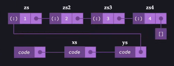
These things in memory are called closures. A closure is an object in memory that contains:
- A pointer to some code that implements the function it represents (not shown)
- A pointer to all the free variables that are in scope for that definition
- A free variable is any variable in scope that is not a parameter
The closures form a graph, where the closures all point to each other.
Another example, using map:
map :: (a -> b) -> [a] -> [b]
map _ [] = []
map f (x:xs) = f x : map f xs
-- removing all syntactic sugar, done by compiler
map = \f -> \arg ->
case arg of
[] -> []
(x: xs) -> let
y = f x
ys = map f xs
in (y:ys)
Using this definition of map to evaluate the expression from before (length (take 2 (map even [1,2,3,4]))):
let
zs4 = 4:[]
zs3 = 3:zs4
zs2 = 2:zs3
zs = 1:zs2
xs = map even zs
ys = take 2 xs
in length ys
-- new closures allocated by map, using 2nd case of map function
let
zs4 = 4:[]
zs3 = 3:zs4
zs2 = 2:zs3
zs = 1:zs2
y0 = even 1
ys0 = map even zs2 -- new closures
xs = y0 : ys -- updated to be a cons cell
ys = take 2 xs
in length ys
The graph of closures representing this:
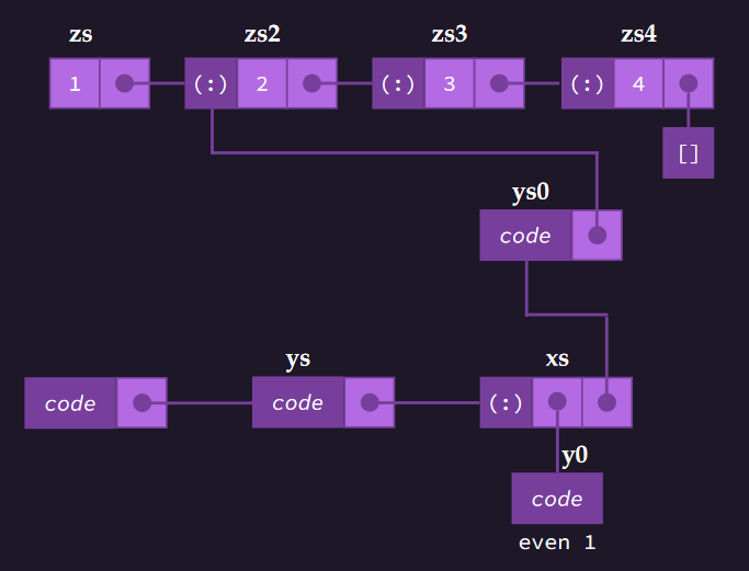
Strictness in Haskell
Things can be evaluated strictly in haskell, if you want. This is prefereable in some cases for performance reasons. The \$! operator forces strict function application. The version of the function below forces the recursive call to be evaluated first.
fac' :: Int -> Int -> Int
fac' 0 m = m
fac' n m = (fac' \$! (n-1)) (n*m)
Infinite Data Structures
Laziness means data structures can be infinite in haskell. This is also facilitated by the lack of call stack, as there is no "max recursion depth" like in strict languages.
from :: Int -> [Int]
from n = n : from (n+1)
This function builds an infinite list of a sequence of Ints, starting with the Int passed. An example usage, showing how lazy evaluation works with it:
take 3 (from 4)
=> take 3 (4 : from 5)
=> 4 : take 2 (from 5)
=> 4 : take 2 (5 : from 6)
=> 4 : 5 : take 1 (from 6)
=> 4 : 5 : take 1 (6 : from 7)
=> 4 : 5 : 6 : take 0 (from 7)
=> 4 : 5 : 6 : []
=> [4,5,6]
The infinite evaluation is short-circuited, as the compiler knows it only needs the first 3 elements.
Reasoning About Programs
Haskell can use normal software testing methods to verify correctness, but because haskell is a pure language, we can do better and formally prove properties of our functions and types.
Natural Numbers
Natural numbers can be defined as data Nat = Z | S Nat in haskell. Alternatively, using mathematical notation, this can be written . Addition can then be defined recursively:
add :: Nat -> Nat -> Nat
add Z m = m
add (S n) m = S (add n m)
Addition has certain properties which must hold true:
- Left identity:
∀m :: Nat, add Z m == m - Right identity:
∀m :: Nat, add m Z == m - Associativity:
∀x y z :: Nat, add x (add y z) == add (add x y) z
These can be proven using equational reasoning, which proves that an equality holds in all cases. Generally, either a property can be proved by applying and un-applying either side of an equation, and/or by induction.
To prove the left identity is easy, as it is an exact match of one of our equations for add:
add Z m
-- applying add
= m
The right identity is a little harder, as we can't just directly apply one of our equations. We can instead induct on m. First, the base case:
add Z Z
-- applying add
= Z
Using the induction hypothesis add m Z = m, we need to show the inductive step holds for S m (m+1):
add (S m) Z
-- applying add
= S (add m Z)
-- applying induction hypothesis
= S m
This proves the right identity. To prove associativity we will again use induction, this time on x. The base case is add Z (add y z):
add Z (add y z)
-- applying add
= add y z
-- un-applying add
= add (add Z y) z
The proof holds for x = Z. Here, the proof was approached from either end to meet in the middle, but written as a single list of operations for clarity. Sometimes it is easier to do this and work from either direction, especially when un-applying functions as it is more natural.
The induction hypothesis is add x (add y z) == add (add x y) z, and can be assumed. We need to prove the inductive step add (S x) (add y z) == add (add (S x) y) z:
add (S x) (add y z)
-- applying add
= S (add x (add y z))
-- applying induction hypothesis
= S (add (add x y ) z)
-- un-applying add
= add (S (add x y)) z
-- un-applying add
= add (add (S x) y) z
This proves associativity.
Induction on Lists
We can induct on any recursive type, including lists: data List a = Empty | Cons a (List a). Using this definition, we can prove map fusion. Map fusion states that we can turn multiple consecutive map operations into a single one with composed functions:
map f (map g xs) = map (f.g) xs∀f :: b -> c∀g :: a -> b∀xs :: [a]
The definitions of map and . may be useful:
map :: (a -> b) -> [a] -> [b]
map f [] = []
map f (x:xs) = f x : map f xs
(.) :: (b -> c) -> (a -> b) -> a -> c
(.) f g x = f (g x)
Map fusion can be proved by induction on xs. The base case is map f (map g []) = map (f.g) []:
map f (map g [])
-- applying map
= map f []
-- applying map
= []
-- un-applying map
= map (f.g) []
Using the induction hypothesis map f (map g xs) = map (f.g) xs, we can prove the inductive case map f (map g (x : xs)) = map (f.g) (x : xs):
map f (map g (x : xs))
-- applying map
= map f (g x : map g xs)
-- applying map
= f (g x) : map f (map g xs)
-- induction hypothesis
= f (g x) : map (f.g) xs
-- un-applying (.)
= (f.g) x : map (f.g) xs
-- un-applying map
= map (f.g) (x : xs)
Proving a Compiler
Given a simple expression language:
data Expr = Val Int | Plus Expr Expr
And a simple instruction set:
data Instr = Push Int | Add
type Program = [Instr]
type Stack = [Int]
We can write an exec function as an interpreter for our instruction set:
exec :: Program -> Stack -> Stack
exec [] s = s
exec (Push n : p) s = exec p (n : s)
exec (Add : p) (y : x : s) = exec p (x + y : s)
An eval function to evaluate our expressions:
eval :: Expr -> Int
eval (Val n) = n
eval (Plus l r) = eval l + eval r
And a comp function as a compiler for our Expr language to our Instr instruction set:
comp :: Expr -> Program
comp (Val n) = [PUSH n]
comp (Plus l r) = comp l ++ comp r ++ [ADD]
Our compiler will be considered correct if for any expression, evaluating it yields the same result as compiling and then executing it:
∀ e :: Expr, s :: Stack . eval e : s == exec (comp e) s
This can be proved by induction on e. The base case for Expr is for Vals, and we want to show that eval (Val n) s == exec (comp (Val n)) s. This time, we start with the RHS:
exec (comp (Val n)) s
-- applying comp
= exec [Push n] s
-- applying exec
= exec [] (n : s)
-- applying exec
= (n : s)
-- unappplying eval
= eval (Val n) s
Our inductive case to be proved is eval (Plus l r) s == exec (comp (Plus l r)) s. Since the Plus constructor has two values of type Expr, there are two induction hypotheses:
- for
l:eval l : s == exec (comp l) s - for
r:eval r : s == exec (comp r) s
exec (comp (Plus l r)) s
-- applying comp
= exec (comp l ++ comp r ++ [Add]) s
-- distributivity of (++)
= exec (comp l ++ (comp r ++ [Add])) s
-- distributivity lemma
= exec (comp r ++ [Add]) (exec (comp l) s)
-- distributivity lemma
= exec [Add] (exec (comp r) (exec (comp l) s))
-- induction hypothesis
= exec [Add] (exec (comp r) (eval l : s))
-- induction hypothesis
= exec [Add] (eval r : (eval l : s))
-- applying exec
= exec [] ((eval l + eval r) : s)
-- applying exec
= (eval l + eval r) : s
-- un-applying exec
= eval (Plus l r) s
The proof holds, but relies on a lemma proving the distributivity of the exec function, which states that executing a program where a list of instructions xs is followed by a list of instructions ys is the same as first executing xs and then executing ys with the stack that results from executing xs: ∀ xs ys::Program, s::Stack . exec (xs++ys) s == exec ys (exec xs s).
This can be proved by induction on xs. The base case is the empty list []: exec ([] ++ ys) s == exec ys (exec [] s):
exec ys (exec [] s)
-- applying exec
= exec ys s
-- un-applying (++)
= exec ([] ++ ys) s
The induction hypothesis is exec (xs++ys) s == exec ys (exec xs s). The inductive step is exec ((x : xs) ++ ys) s == exec ys (exec (x : xs) s). As x could be either Push x or Add, we perform case analysis on x, first with the case where x = Push n:
exec ys (exec (Push n : xs) s)
-- applying exec
= exec ys (exec xs (n : ns))
-- induction hypothesis
= exec (xs ++ ys) (n : s)
-- un-applying exec
= exec (Push n : (xs ++ ys)) s
-- un-applying (++)
= exec ((Push n : xs) ++ ys) s
The inductive step holds for the Push n case. The Add case:
exec ys (exec (Add : xs) s)
-- assuming stack has at least 2 elements
exec ys (exec (Add : xs) (b : a : s'))
-- applying exec
exec ys (exec xs (a + b : s'))
-- induction hypothesis
exec (xs ++ ys) (a + b : s')
-- un-applying exec
exec (Add : (xs ++ ys)) (b : a : s')
-- un-applying (++)
exec ((Add : xs) ++ ys) (b : a : s')
-- assumption
exec ((Add : xs) ++ ys) s
This proves the inductive case for the Add instruction, and therefore the proof for the distributivity of exec lemma, which supported our initial proof of the correctness of our compiler.
Functors & Foldables
The \$ Operator
The \$ operator is an operator for function application. It has signature:
(\$) :: (a -> b) -> a -> b
f \$ x = f x
At first it doesn't look like it does much, but it is actually defined as infixr 0 meaning it is:
- An infix operator with right associativity
- Has the lowest precedence possible.
In contrast, normal function application is left associative and has the highest precedence possible. Practically, this means it can be used where you would otherwise have to use parentheses, to make code a lot cleaner. Some examples:
-- elem finds if an item x is contained in the list xs
elem :: Eq a => a -> [a] -> Bool
elem x xs = not (null (filter (==x) xs))
-- rewritten, without parentheses
elem x xs = not \$ null \$ filter (==x) xs
-- or using function composition (.)
elem x = not . null . filter (==x)
Another example, shown along with a trace of it's reduction:
map (\$ 4) [even, odd]
=> (even $ 4) : map (\$ 4) [odd]
=> (even \$ 4) : (odd \$ 4) : []
=> True : (odd \$ 4) : []
=> True : False : []
=> [True, False]
Foldables
It has already been shown how many examples of recursive functions can be rewritten with a fold. folding is a an example of a useful design pattern in functional programming.
A Trip to Michael's Tree Nursery
Binary trees are recursive data structures, that can be recursively operated on (much like lists). The example below shows a simple definition of a binary tree along with some functions to operate on it.
-- our binary tree type
data BinTree a = Leaf | Node (BinTree a) a (BinTree a)
deriving Show
-- simple recursive functions
-- how big is the tree?
size :: BinTree a -> Int
size Leaf = 0
size Node (l _ r) = 1 + size l + size r
-- is x contained within the tree?
member:: Eq a => a -> BinTree a -> Bool
member _ Leaf = False
member x (Node l y r) = x == y || member x l || member x r
-- what is the sum of all the Nums in the tree
tsum :: Num a => BinTree a -> a
tsum Leaf =0
tsum (Node l n r) = n + tsum l + tsum r
These are all recursive functions operating on a tree, and can be generalised by defining our own version of a fold for trees, dubbed toldr. Note the similarities between foldr and toldr.
toldr :: (a -> b -> b) -> b -> BinTree a -> b
toldr f z Leaf = z
toldr f z (Node l x r) = f x (toldr f (toldr f z r) l)
tsum :: Num a => BinTree a -> a
tsum = toldr (+) 0
member :: Eq a => a -> BinTree a -> Bool
member x = toldr (\y r -> x==y || r) False
size :: BinTree a -> Int
size = toldr(\_ r -> 1 + r) 0
The Foldable Typeclass
This abstraction does actually exist in the standard libary, as a typeclass. A type can be an instance of Foldable (like lists), which then allows foldr to be used on it.
class Foldable t where
foldr :: (a -> b -> b) -> b -> t a -> b
-- for lists
-- exists in prelude
instance Foldable [] where
foldr f z [] = z
foldr f z (x:xs) = f x (foldr f z xs)
-- for our bintree
instance Foldable BinTree where
foldr _ z Leaf = z
foldr f z (Node l x r) = f x (foldr f (foldr f z r) l)
This instance of Foldable for BinTree can now be used to generalise our functions that operate on it:
sum :: (Foldable t, Num a) => t a -> t
sum = foldr (+) 0
elem :: (Foldable t, Eq a) => a -> t a -> Bool
elem x = foldr (\y r -> x==y || r) False
length :: Foldable t => t a -> Int
length = foldr (\_ r -> 1 + r) 0
These methods are actually part of the Foldable typeclass, so when defining an instance of Foldable on some type, you get them for free, and they are polymorphic over all foldable types.
Foldable is also a derivable typeclass using the language extension -XDeriveFoldable, so all of this can be derived automatically.
Functors
Bringing back our safediv function from previously:
data Maybe a = Nothing | Just a
safediv :: Int -> Int -> Maybe Int
safediv _ 0 = Nothing
safediv x y = Just (x `div` y)
divAndAdd :: Int -> Int -> Maybe Int
divAndAdd x y = 5 + safediv x y -- doesn't work, type error
-- using a case statement
divAndAdd x y = case safediv x y of
Nothing -> Nothing
Just r -> Just (5+r)
-- bit messy
The pattern of applying a function a value within a Maybe can be generalise. Defining a function pam to do this for us:
pam :: (a -> b) -> Maybe a -> Maybe b
pam _ Nothing = Nothing
pam f (Just x) = Just (f x)
-- much nicer!
divAndAdd :: Int -> Int -> Maybe Int
divAndAdd x y = pam (5+) (safediv x y)
It would be nice if there was some way to generalise the pattern of applying a function to element(s) in a container. The Functor typeclass does this for us. A type is a functor if we can apply a function to it. Lists are functors, as that is what the map function does. Maybe and BinTrees are also functors.
class Functor f where
fmap :: (a -> b) -> f a -> f b
instance Functor [] where
fmap = map
instance Functor Maybe where
fmap f Nothing = Nothing
fmap f (Just x) = Just (f x)
instance Functor BinTree where
fmap f (Leaf x) = Leaf (f x)
fmap f (Node lr ) = Node (fmap f l) (fmap f r)
Functors can be thought of as "boxes", and when given a function, will apply it to the value in the box, and return the result in the same box. Some examples of definitions using functors:
-- increases all Ints in the "box" by 5
incByFive :: Functor f => f Int -> f Int
incByFive = fmap (+5)
-- applies the odd function to all Ints in the box
odds :: Functor f => f Int -> f Bool
odds = fmap odd
-- redefining using fmap
divAndAdd :: Functor f => Int -> Int -> Maybe Int
divAndAdd x y = fmap (5+) (safediv x y)
Functor is also another typeclass that can be derived by GHC, using the -XDeriveFunctor extension.
The <\$> Operator
An operator that is essentially just an infix version of the fmap function.
infixl 4 <\$>
(<\$>) :: Functor f => (a -> b) -> f a -> f b
(<\$>) = fmap
fmap (replicate 6) (safediv 8 4)
== replicate 6 <\$> safediv 8 4
=> Just [2,2,2,2,2,2]
-- redefining using <\$>
divAndAdd :: Functor f => Int -> Int -> Maybe Int
divAndAdd x y = (5+) <\$> (safediv x y)
Functor Laws
There are certain laws that functors must obey for their properties to hold. A type f is a functor if there exists a function fmap :: (a-> b) -> f a -> f b , and the following laws hold for it:
fmap id = id- If the values in the functor are mapped to themselves, the result will be an unmodified functor
fmap (f.g) = (fmap f) . (fmap g)- The fusion law
- If two
fmaps are applied one after the other, the result must be the same as a singlefmapwhich applies the two functions in turn
- These laws imply that a data structure's "shape" does not change when
fmapped
Applicative Functors
Kinds
- For the compiler to accept a program, it must be well typed
- Kinds are the "types of types"
- Types are denoted with
expression :: type- eg
True :: Bool
- eg
- Kinds are denoted the same:
type :: kindBool :: *
- The compiler infers kinds of types the same way it infers types of expressions
*is the kind of typesBool :: *becauseBoolhas no type parametersdata Bool = True | False
Maybeis parametrised over some typea, so the kind signatureMaybe :: * -> *means that if given a type as an argument to the type constructorJust, it will give back some other type of kind*[] :: * -> *[]is the type constructor for lists
Kinds are important when defining typeclasses. Take Functor, for example:
class Functor f where
fmap :: (a -> b) -> f a-> f b
This definition shows that the type f is applied to one argument (f a), so f :: * -> *
-- Maybe :: * -> *
instance Functor Maybe where
fmap f Nothing = Nothing
fmap f (Just x) = Just (f x)
-- invalid
-- Maybe a :: *
-- As the type is already applied to a
instance Functor (Maybe a) where
fmap f Nothing = Nothing
fmap f (Just x) = Just (f x)
The Either Type
Either is usually used to represent the result of a computation when it could give one of two results. Right is used to represent success, and a is the wanted value. Left is used to represent error, with e as some error code/message.
data Either e a = Left e | Right a
Left :: e -> Either e a
Right :: a -> Either e a
Either has kind * -> * -> *, as it must be applied to two types e and a before we get some other type.
Only types of kind * -> * can be functors, so we need to apply Either to one argument first. The functor instance for Either applies the function to the Right value.
instance Functor (Either e) where
fmap :: (a -> b) -> Either e a -> Either e b
fmap f (Left x) = Left x
fmap f (Right y) = Right (f y)
The Unit Type ()
()is called the unit type() :: ()(), the unit value, has type()()is the only value of type()
- Can be thought of as defined
data () = () - Or an empty tuple
Semigroups and Monoids
A type is a semigroup if it has some associative binary operation defined on it. This operator (<>) is the "combine" operator.
class Semigroup a where
(<>) :: a -> a -> a
instance Semigroup [a] where
-- (<>) :: [a] -> [a] -> [a]
(<>) = (++)
instance Semigroup Int where
-- (<>) :: Int -> Int -> Int
(<>) = (+)
A type is a monoid if it is a semigroup that also has some identity value, called mempty:
class Semigroup a => Monoid a where
mempty ::a
instance Monoid [a] where
-- mempty :: [a]
mempty = []
instance Monoid Int where
-- mempty :: Int
mempty = 0
Applicatives
Applicative Functors are similar to normal functors, except with a slightly different type definition:
class Functor f => Applicative f where
pure :: a -> f a
<*> :: f (a -> b) -> f a -> f b
The typeclass defines two functions:
purejust lifts the valueainto the "box"<*>(the apply operator) takes some function (a -> b) in a boxf, and applies it to a valueain a box, returning the result in the same box.- "box" is a rather loose analogy. It is more accurate to say "computational context".
Different contexts for function application:
-- vanilla function application
(\$) :: (a -> b) -> a -> b
-- Functor's fmap
(<\$>) :: Functor f => (a -> b) -> f a -> f b
-- Applicative's apply
(<*>) :: Applicative f => f (a -> b) -> f a -> f b
Maybe and Either e are both applicative functors:
instance Applicative Maybe where
pure x = Just x
Nothing <*> _ = Nothing
(Just f) <*> x = f <\$> x
instance Applicative (Either e) where
pure = Right
Left err <*> _ = Left err
Right f <*> x = f <\$> x
The "context" of both of these types is that they represent error. All data flow in haskell has to be explicit due to its purity, so these types allow for the propagation of error.
Another example of an applicative functor is a list:
instance Applicative [] where
pure x = [x]
fs <*> xs = [f x | f <- fs, x <- xs]
Every function in the left list is applied to every function in the right:
[f, g] <*> [x, y, z]
=> [f x, f y, f z, g x, g y, g z]
g <\$> [x,y] <*> [a,b,c]
=> [g x, g y] <*> [a,b,c]
=> [g x a, g x b, g x c, g y a, g y b, g y c]
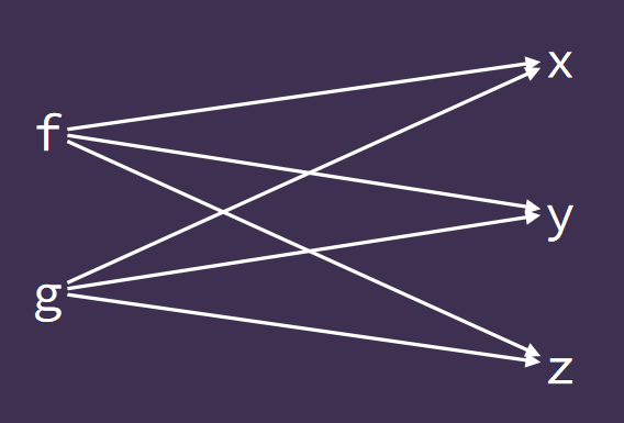
The context represented by lists is nondeterminism, ie a function f given one of the arguments [x, y, z] could have result [f x, f y, f z].
Applicative Laws
Applicative functors, like normal functors, also have to obey certain laws:
pure id <*> x = x- The identity law
- applying pure id does nothing
pure f <*> pure x = pure (f x)- Homomorphism
purepreserves function application
u <*> pure y = pure (\$ y) <*> u- Interchange
- Applying something to a pure value is the same as applying pure ($ y) to that thing
pure (.) <*> u <*> v <*> w = u <*> (v <*> w)- Composition
- Function composition with
(.)works within apurecontext.
Left and Right Apply
<* and *> are two more operators, both defined automatically when <*> is defined.
const :: a -> b -> a
const x y = x
flip :: (a -> b -> c) -> b -> a -> c
flip f x y = f y x
(<*) :: Applicative f => f a -> f b -> f a
a0 <* a1 = const <\$> a0 <*> a1
(*>) :: Applicative f => f a -> f b -> f b
a0 *> a1 = flip const <\$> a0 <*> a1
In simple terms *> is used for sequencing actions, discarding the result of the first argument. <* is the same, except discarding the result of the second.
Just 4 <* Just 8
=> const <\$> Just 4 <*> Just 8
=> Just (const 4) <*> Just 8
=> Just (const 4 8)
=> Just 4
Just 4 <* Nothing
=> const <\$> Just 4 <*> Nothing
=> Just (const 4) <*> Nothing
=> Nothing
Just 4 *> Just 8
=> flip const <\$> Just 4 <*> Just 8
=> Just (flip const 4) <*> Just 8
=> Just (flip const 4 8)
=> Just (const 8 4)
=> Just 8
Nothing *> Just 8
=> Nothing
These operators are perhaps easier to understand in terms of monadic actions:
as *> bs = do as
bs
as *> bs = as >> bs
as <* bs = do a <- as
bs
pure a
Example: Logging
A good example to illustrate the uses of applicative functors is logging the output of a compiler. If we have a function comp that takes some Expr type, representing compiler input, and returns some Program type, representing output :
comp :: Expr -> Program
comp (Val n) = [PUSH n]
comp (Plus l r) = comp l ++ comp r ++ [ADD]
-- extending to return a String for a log
comp :: Expr -> (Program, [String])
comp (val n) = ([PUSH n],["compiling a value"])
comp (Plus l r) = (pl ++ pr ++ [ADD], "compiling a plus" : (ml ++ mr))
where (pl, ml) = comp l
(pr, mr) = comp r
This is messy and not very clear what is going on. There is a much nicer way to do this, using the Writer type:
-- w is the "log"
-- a is the containing type (the type in the "box")
data Writer w a = MkWriter (a,w)
--type of MkWriter
MkWriter :: (a,w) -> Writer w a
-- kind of Writer type
Writer :: * -> * -> *
instance Functor (Writer w) where
-- fmap :: (a -> b) -> Writer w a -> Writer w b
fmap f (MkWriter (x,o)) = MkWriter (f x, o) -- applies the function to the x value
-- a function to write a log
-- generates a new writer with a msg and unit type in it's box
writeLog :: String -> Writer [w] ()
writeLog msg = MkWriter((), [msg])
Using this to redefine comp:
comp :: Expr -> Writer [String] Program
comp (Val n) = MkWriter ([PUSH n], m)
where (MkWriter (_, m)) = writeLog "compiling a value"
comp (Plus l r) = MkWriter (pl ++ pr ++ [ADD], m ++ ml ++ mr)
where (MkWriter (pl, ml)) = comp l
(MkWriter (pr, mr)) = comp r
(MkWriter (_, m)) = writeLog
This definition of comp combines the output using Writer, but is messy as it uses pattern matching to deconstruct the results of the recursive calls and then rebuild them into the result. It would be nice if there was some way to implicitly keep track of the log messages.
We can define an instance of the Applicative typeclass for Writer to do this. There is the additional constraint that w must be an instance of Monoid, because we need some way to combine the output of the log.
instance Monoid w => Applicative (Writer w) where
--pure :: a -> Writer w a
pure x = MkWriter (x, mempty)
-- <*> Monoid w => Writer w (a -> b) -> Writer w a -> Writer w b
MkWriter (f,o1) <*> MkWriter (x,o2) = MkWriter (f x, o1 <> o2)
-- f is applied to x, and o1 and o2 are combined using their monoid instance
Using this definition, the comp function can be tidied up nicely using <*>
comp :: Expr -> Writer [String] Program
comp (Val n) = writeLog "compiling a value" *> pure [PUSH n]
comp (Plus l r) = writeLog "compiling a plus" *>
((\p p' -> p ++ p' ++ [ADD]) <\$> comp l <*> comp r)
The first pattern uses *>. Recall that *> does not care about the left result, which in this case is the unit type, so only the result of the right Writer is used, which is the [PUSH n] put into a Writer by pure, with a mempty, or [] as the logged value.
The second pattern applies the anonymous function (\p p' -> p ++ p' ++ [ADD]) to the result of the recursive calls. The lambda defines how the results of the recursive calls are combined together, and the log messages are automatically combined by the definition of <*>. *> is used again to add a log message to the program.
Monads
ṱ̴̹͙̗̣̙ͮ͆͑̊̅h̸̢͔͍̘̭͍̞̹̀ͣ̅͢e̖̠ͫ̒ͦ̅̉̓̓́͟͞ ͑ͥ̌̀̉̐̂͏͚̤͜f͚͔͖̠̣͚ͤ͆ͦ͂͆̄ͥ͌o̶̡̡̝͎͎̥͖̰̭̠̊r̗̯͈̀̚b̢͙̺͚̅͝i̸̡̱̯͔̠̲̿dͧ̈ͭ̑҉͎̮d̆̓̂̏̉̏͌͆̚͝͏̺͓̜̪͓e̎ͯͨ͢҉͙̠͕͍͉n͇̼̞̙͕̮̣͈͓ͨ͐͛̽ͣ̏͆́̓ ̵ͧ̏ͤ͋̌̒͘҉̞̞̱̲͓k͔̂ͪͦ́̀͗͘n͇̰͖̓ͦ͂̇̂͌̐ȯ̸̥͔̩͒̋͂̿͌w̞̟͔̙͇̾͋̅̅̔ͅlͧ͏͎̣̲̖̥ẻ̴̢̢͎̻̹̑͂̆̽ͮ̓͋d̴̪͉̜͓̗̈ͭ̓ͥͥ͞g͊̾̋̊͊̓͑҉͏̭͇̝̰̲̤̫̥e͈̝̖̖̾ͬ̍͢͞
Monads are another level of abstraction on top of applicatives, and allow for much more flexible and expressive computation. Functors => Applicatives => Monads form a hierarchy of abstractions.
The Monad typeclass
class Applicative m => Monad m where
(>>=) :: m a -> (a -> m b) -> m b
return :: a -> m a
return = pure
The >>= operator is called bind, and applies a function that returns a wrapped value, to another wrapped value.
- The left operand is some monad containing a value
a - the right operand is a function of type
a -> m b, ie it takes someaand returns a monad containing something of typeb - The result is a monad of type
b
The operator can essentially be thought of as feeding the wrapped value into the function, to get a new wrapped value. x >>= f unwraps the value in x from it, and applies the function to f to it. Understanding bind is key to understanding monads.
return is just the same as pure for applicatives, lifting the value a into some monadic context.
Some example monad instances:
instance Monad Maybe where
Nothing >>= _ = Nothing
Just x >>= f = f x
instance Monad (Either e) where
Left l >>= _ = Left l
Right r >>= f = f r
pure = Right
instance Monad [] where
xs >>= f = concat (map f xs)
Monads give effects: composing computations sequentially using >>= has an effect. With the State Monad this effect is "mutation". With Maybe and Either the effect is that we may raise a failure at any step. Effects only happen when we want them, implemented by pure functions.
Monad Laws
For a type to be a monad, it must satisfy the following laws:
return a >>= h = h a- Left identity
m >>= return = m- Right identity
(m >>= f) >>= g = m >>= (\x -> f x >>= g)- Associativity
Example: Evaluating an Expression
A type Expr is shown below that represents a mathematical expression, and an eval function to evaluate it. Note that it is actually unsafe and could crash at runtime due to a div by 0 error. The safediv function does this using Maybe.
data Expr = Val Int | Add Expr Expr | Div Expr Expr
eval :: Expr -> Int
eval (Val n) = n
eval (Add l r) = eval l + eval r
eval (Div l r) = eval l `div` eval r
safediv :: Int -> Int -> Maybe Int
safediv x 0 = Nothing
safediv x y = Just (x `div` y)
If we want to use safediv with eval, we need to change it's type signature. The updated eval is shown below using applicatives to write the function cleanly and propagate any errors:
eval :: Expr -> Maybe Int
eval (Val n) = Just n
eval (Add l r) = (+) <\$> eval l <*> eval r
eval (Div l r) = safediv <\$> eval l <*> eval r
If any recursive calls return a Nothing, the entire expression will evaluate to Nothing. Otherwise, the <\$> and <*> will evaluate the expression within the Maybe context. However, this is still wrong as the last expression now has type of Maybe (Maybe Int). This can be fixed using >>=. Note the use of lambdas.
eval (Div l r) = eval l >>= \x ->
eval r >>= \y ->
x `safediv` y
The Expr type can be extended to include a conditional expression, where If Condition True False`.
data Expr = Val Int
| Add Expr Expr
| Div Expr Expr
| If Expr Expr Expr
eval :: Expr -> Maybe Int
eval (Val n) = Just n
eval (Add l r) = eval l >>= \x ->
eval r >>= \y ->
Just (x+y)
eval (Div l r) = eval l >>= \x ->
eval r >>= \y ->
x `safediv` y
eval (If c t f) = ifA <\$> eval c <*> eval t <*> eval f
where ifA b x y = if b /= 0 then x else y
With this definition using applicatives, both branches of the conditional branch are evaluated. If there is an error in the false branch, the whole expression will fail. Here, using bind, the semantics are correct.
eval' (If c t f) = eval' c >>= \b ->
if b /= 0 then eval t else eval f
<*> vs >>=
Bind is a much more powerful abstraction than apply:
<*> :: m (a -> b) -> m a -> m b
(>>=) :: m a -> (a -> m b) -> m b
- Apply operates on functions already inside a context
- This function can't determine anything to do with the context
- With a
Maybe, it can't determine if the overall expression returnsNothingor not
- Bind takes a function that returns a context, and can therefore can determine more about the result of the overall expression
- It knows if it's going to return
Nothing
- It knows if it's going to return
do Notation
Notice the pattern of >>= being used with lambdas a fair amount. This can be tidied up with some nice syntactic sugar, called do notation. Rewriting the earlier example:
eval :: Expr -> Maybe Int
eval (Val n) = return n
eval (Add l r) = do
x <- eval l
y <- eval r
return (x+y)
eval (Div l r) = do
x <- eval l
y <- eval r
x `safediv` y
This looks like imperative code, but is actually using monads behind the scenes. The arrows bind the results of the evaluation to some local definition, which can then be referred to further down the block.
- A block must always end with a function call that returns a monad -
- usually
return, butsafedivis used too
- usually
- If any of the calls within the
doblock shown returnsNothing, the entire block will short-circuit to aNothing.
Example: The Writer Monad
The example of Writer as an applicative instance can be extended to make it a Monad instance.
data Writer w a = MkWriter (a,w)
instance Functor (Writer w) where
-- fmap :: (a -> b) -> Writer w a -> Writer w b
fmap f (MkWriter (x,o)) = MkWriter(f x, o)
instance Monoid w => Applicative (Writer w) where
-- pure :: Monoid w => a -> Writer w a
pure x = MkWriter (x, mempty)
-- <*> :: Monoid w => Writer w (a -> b) -> Writer w a -> Writer w b
MkWriter (f,o1) <*> MkWriter (x,o2) = MkWriter (f x, o1 <> o2)
instance Monoid w => Monad (Writer w) where
-- return :: Monoid w => a -> Writer w a
return = MkWriter (x, mempty) --pure
(Writer (x, o1)) >>= f = MkWriter (y, o2 <> o1)
where (MkWriter (y,o2)) = f x
Bind for Writer applies the function to the x value in the writer, then combines the two attached written values, and return the new value from the result of f x along with the combined values.
Now we have a monad instance for the Writer monad, we can rewrite our comp function with do notation:
comp' :: Expr -> Writer [String] Program
comp' (Val n) = do
writeLog "compiling a value"
pure [PUSH n]
comp' (Plus l r) = do writeLog "compiling a plus"
pl <- comp l
pr <- comp r
pure (pl ++ pr ++ [ADD])
Type Level Programming
Type level programming is about encoding more information in our types, so make them more descriptive. The more descriptive types are, the easier it is to avoid runtime errors, as the type checker can do more at compile time.
The GHC language extensions used here are:
-XDataKinds-XGATDs-XKindSignatures-XScopedTypeVariables-XTypeFamilies
Type Promotion
As we already know, types have kinds:
Bool :: *Maybe :: * -> *[] :: * -> *State :: * -> * -> *
Also recall that we have to partially apply type constructors with kinds greater than * -> * to use them as monads:
-- Maybe :: * -> *
instance Monad Maybe where
...
-- State :: * -> * -> *
instance Monad (State s) where
...
-- Either :: * -> * -> *
instance Monad Either where
... -- type error
instance Monad (Either e) where
... -- works
Type Promotion is used to define our own kinds. The DataKinds extension allows for this. Without DataKinds, data Bool = True | False gives us two constructors, True and False. At the three levels in haskell:
- At the kind-level:
* - At the type-level
Bool - At the value-level:
TrueorFalse
With DataKinds, we also get the following two new types, both of kind Bool:
'True :: Bool'False :: Bool
The value constructors True and False have been promoted to the type level as 'True and 'False. A new kind is introduced too, Bool instead of just *. We now have booleans at the type level.
DataKinds promotes all value constructors to type constructors, and all type constructors to kinds.
Another example, recursively defined natural numbers. Zero is 0, and Succ Nat is Nat + 1.
data Nat = Zero | Succ Nat
-- values :: types
Zero :: Nat
Succ :: Nat -> Nat
-- types :: kinds
'Zero :: Nat
'Succ :: Nat -> Nat
Generalised Algebraic Data Types
GADTs allow for more expressive type definitions. Normal ADT syntax:
data Bool = True | False
-- gives two values
True :: Bool
False :: Bool
Usually, we define the type and its values, which yields two value constructors. With a GADT, we explicitly specify the type of each data constructor:
data Bool where
True :: Bool
False :: Bool
data Nat where
Zero :: Nat
Succ :: Nat -> Nat
The example below defines a recursively defined Vector type.
-- Normally
data Vector a = Nil | Cons a (Vector a)
-- GADT
data Vector a where
Nil :: Vector a
Cons :: a -> Vector a -> Vector a
Example: A Safe Vector
The vector definition above can use another feature, called KindSignatures, to put more detail into the type of the GADT definition:
data Vector (n :: Nat) a where
Nil :: Vector n a
Cons :: a -> Vector n a -> Vector n a
This definition includes an n to encode the size of the vector in the type. n is a type of kind Nat, as defined above. The values and types were promoted using DataKinds. The type variable n can also be replaced with concrete types:
data Vector (n :: Nat) a where
Nil :: Vector `Zero a
Cons :: a -> Vector n a -> Vector (`Succ n) a
-- example
cakemix :: Vector ('Succ ('Succ Zero)) String
cakemix = Cons "Fish-Shaped rhubarb" (Cons "4 large eggs" Nil)
This further constrains the types to make the types more expressive. Now we have the length of the list expressed at type level, we can define a safer version of the head function that rejects zero-length lists at compile time.
vhead :: Vector ('Succ n) a -> a
-- this case will throw an error at compile time as it doesn't make sense
vhead Nil = undefined
vhead (Cons x xs) = x
Can also define a zip function for the vector type that forces inputs to be of the same length. The type variable n tells the compiler in the type signature that both vectors should have the same length.
vzip :: Vector n a -> Vector n b -> Vector n (a,b)
vzip Nil Nil = Nil
vzip (Cons x xs) (Cons y ys) = Cons (x,y) (vzip xs ys)
Singleton types
Singletons are types with a 1:1 correspondence between types and values. Every type has only a single value constructor. The following GADT is a singleton type for natural numbers. The (n :: Nat) in the type definition annotates the type with it's corresponding value at type level. The type is parametrised over n, where n is the value of the type, at type level.
data SNat (n :: Nat) where
SZero :: SNat 'Zero
SSucc :: Snat n -> SNat ('Succ n)
-- there is only one value of type SNat 'Zero
szero :: SNat 'Zero
szero = SZero
-- singleton value for one and it's type
sone :: SNat ('Succ 'Zero)
sone = SSucc SZero
stwo :: SNat ('Succ ('Succ Zero))
sone = SSucc sone
There is only one value of each type. The data is stored at both the value and type level.
This can be used to define a replicate function for the vector:
vreplicate :: SNat n -> a -> Vector n a
vreplicate SZero x = Nil
vreplicate (SSucc n) x = Cons x (vreplicate n x)
The length of the vector we want is SNat n at type level, which is a singleton type. This allows us to be sure that the vector we are outputting is the same size as what we told it, making sure this type checks.
Proxy Types & Reification
We are storing data at the type level, which allows us to access the data at compile time and statically check it. If we want to access that data at runtime, for example to find the length of a vector, we need a proxy type. Proxy types allow for turning type level data to values, ie turning a type level natural number (Nat) into an Int. Haskell has no types at runtime (due to type erasure), so proxies are a hack around this.
-- a type NatProxy parametrised over some type a of kind Nat
data NatProxy (a :: Nat) = MkProxy
-- NatProxy :: Nat -> *
-- MkProxy :: NatProxy a
This proxy type is parametrised over some value of type a with kind Nat, but there is never actually any values of type a involved, the info is at the type level. a is a phantom type.
zeroProxy :: NatProxy 'Zero
zeroProxy = MkProxy
oneProxy :: NatProxy ('Succ 'Zero)
oneProxy = MkProxy
These two proxies have the same value, but different types. The Nat type is in the phantom type a at type level.
We can then define a type class, called FromNat, that is parametrised over some type n of kind Nat:
class FromNat (n :: Nat) where
fromNat :: NatProxy n -> Int
The function fromNat takes a NatProxy, our proxy type, and converts it to an int. Instances can be defined for the two types of Nat to allow us to covert the type level Nats to Ints.
-- instance for 'Zero
instance FromNat 'Zero where
-- fromNat :: NatProxy 'Zero -> int
fromNat _ = 0
instance FromNat n => FromNat ('Succ n) where
fromNat _ = 1 + fromNat (MkProxy :: NatProxy n)
The arguments to these functions are irrelevant, as the info is in the types. The variable n refers to the same type variable as in the instance head, using scoped type variables. This hack allows for passing types to functions using proxies, and the converting them to values using reification.
Type Families
Type families allow for performing computation at the type level. A type family can be defined to allow addition of two type-level natural numbers:
type family Add (n :: Nat) (m :: Nat) :: Nat where
Add 'Zero m = m
Add ('Succ n) m = 'Succ (Add n m)
-- alternatively
type family (n :: Nat) + (m :: Nat) :: Nat where
'Zero + m = m
'Succ n + m = 'Succ (n + m)
The type family for (+) is whats known as a closed type family: once it's defined it cannot be redfined or added to. This type family can be used to define an append function for our vector:
vappend :: Vector n a -> Vector m a -> Vector (n+m) a
vappend Nil ys = ys
vappend (Cons x xs) ys = Cons x (vappend xs ys)
Importing GHC.TypeLits allows for the use of integer literals at type level instead of writing out long recursive type definitions for Nat. This means we can now do:
data Vector (n :: Nat) a where
Nil :: Vector 0 a
Cons :: a -> Vector n a -> Vector (n+1) a
vappend Nil Nil :: Vector 0 a
vappend (Cons 4 Nil) Nil :: Vector 1 Int
vappend (Cons 4 Nil) (Cons 8 Nil) :: Vector 2 Int
Associated (Open) Type Families
The definition below defines a typeclass for a general collection of items:
class Collection c where
empty :: c a
insert :: a -> c a -> c a
member :: a -> c a -> Bool
instance Collection [] where
empty = []
insert x xs = x : xs
member x xs = x `elem` xs
However, the list instance will throw an error, as elem has an Eq constraint on it, while the member type from the typeclass doesn't. Another example, defining the red-black tree as an instance of Collection (the tree is defined in one of the lab sheets):
instance Collection Tree where
empty = empty
insert x t = insert t x
member x t = member x t
This will raise two type errors, as both insert and member for the tree need Ord constraints, which Collection doesn't have.
To fix this, we can attach an associated type family to a type class.
class Collection c where
type family Elem c :: *
empty :: c
insert :: a -> c -> c
member :: a -> c -> Bool
For an instance of Collection for some type c, we must also define a case for c for a type level function Elem, this establishing a relation between c and some type of kind *.
We can now define instance for list and tree, where Eq and Ord constraints are placed in instance definition.
instance Eq a => Collection [a] where
type Elem [a] = a
empty = []
insert x xs = x : xs
member x xs = x `elem` xs
instance Ord a => Collection (L.Tree a) where
type Elem (L.Tree a) = a
empty = L.Leaf
insert x t = L.insert t x
member x t = L.member x t
ES191
A (yet incomplete) collection of notes for ES191 Electrical and Electronic Circuits.
This one aims to be fairly comprehensive, so let me know if you think anything is missing.
If you're looking for notes on digital logic, see CS132
Other Useful Resources
- https://www.khanacademy.org/science/electrical-engineering/ee-circuit-analysis-topic/circuit-elements/a/ee-sign-convention
- https://spinningnumbers.org/
- https://www.electronics-tutorials.ws/opamp/opamp_1.html
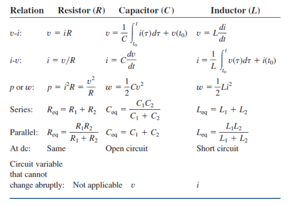
Circuit Symbols and Conventions
Circuits model electrical systems
- Voltage is work done per unit charge
- Potential difference- difference in electrical potential between two points in an electric field
- A force used to move charge between two points in space
- Moving charges produce an electric current
- Moving charges can do electrical work the same way moving objects do mechanical work
- Electrical energy is the capacity to do electrical work
- Electrical power is the rate at which work is done
Resistance
- Resistance is the opposition to the flow of current
- Ohm's Law:
- Resistance is also proportional to the Resistivity of the material
- and are the length and area of the conductor, respectively.
Sources and Nodes
Everything in a circuit can be modelled as either a source, or a node.
Voltage Sources
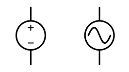
- DC and AC voltage sources
- DC source has positive and negative terminals
- Ideal voltage source has 0 internal resistance (infinite conductance)
- Supplies constant voltage regardless of load
- This is an assumption, is not the case in reality
Current Sources
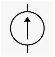
- Ideal current source has infinite resistance (0 conductance)
- Supplies constant current regardless of load
- Also an assumption
- In reality, will have some internal resistance and therefore a maximum power limit
Dependant sources
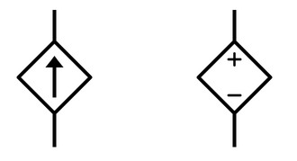
- Diamond-shaped
- Sources depend on values in other parts of the circuit
- Model real sources more accurately
Nodes
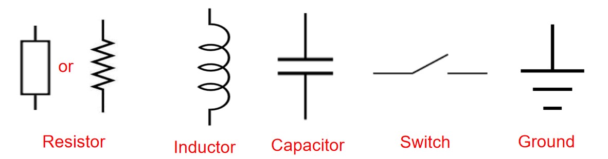
All passive elements: generate no electrical power.
- Resistors provide resistance/impedance in Ohms ()
- Inductors provide inductance in Henries ()
- Capacitors provide capacitance in Farads ()
The voltage rise across an impedance conducting current is in opposition to the flow of current in the impedance.
Basic Conventions
Electrical current always flows from high to low potential.
- If the direction of the current in a circuit is such that it leaves the positive terminal of a voltage source and enters the negative terminal, then the voltage is designated as negative
- If the direction of the current is such that it leaves the negative and enters the positive, then the voltage is positive
- The sign of the loop current is the terminal that it flows into
The power absorbed/produced by a source is .
- A voltage source is absorbing power if it is supplying a negative current
- A voltage source is producing power if it is supplying a positive current
The power dissapated in a resistor is .
Resistors in series and parallel
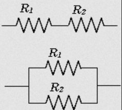
Resistors in series:
Resistors in parallel:
Resistors dissipate electrical power, so there is a drop in voltage accross them, in the direction of current flow. Therefore, the voltage rise is in opposition to the direction of current
Voltage dividers
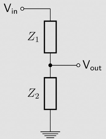
Using two resistors to divide a voltage
In the general case:
Current Dividers
Similar deal to voltage divider
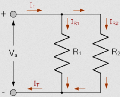
Nodal Analysis
Kirchhoff's Current Law
The sum of currents entering a node is equal to the sum of currents leaving a node.
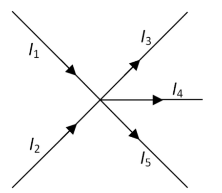
- Currents flowing into a node are denoted as negative
- Currents flowing out of a node are denoted positive
- The sum of currents around a node must always be 0
Nodal Analysis
A technique used to analyse circuits to calculate unknown quantities. Allows the voltage at each circuit node to be calculated, using KCL.
An important point to remember is that the bottom of any circuit diagram is ground (0V), by convention.
Steps
- Choose 1 node as the reference node
- Label any remaining voltage nodes
- Substitute any known voltages
- Apply KCL at each unknown node to form a set of simultaneous equations
- Solve simultaneous equations for unknowns
- Calculate any required values (usually currents)
Generally speaking, there will be a nodal equation for each node, formed using KCL, and then these equations will solve simultaneously.
Example
Calculate the voltages at nodes and .
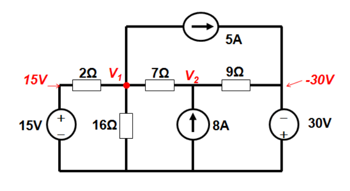
There are 4 currents at
- Flowing from 15V source to accross 2 resistor
- Flowing from to ground accross 16 resistor
- Flowing between and accross 7 resistor
- 5A, from current source
Each current is calculated using ohm's law, which gives the following nodal equation:
When the direction of each current is not known it is all assumed to be positive, and the voltage at the node is labelled as postive, with any other voltages being labelled as negative. Similar can be done for node :
We now have two equations with two unknowns, which can easily be solved.
Admittance Matrices
The system of equations above can also be represented in matrix form
This matrix equation always takes the form .
is known as the Admittance Matrix.
Calculating Power Dissapated
Sometimes, it is required that the power dissapated by voltage/current sources is calculated. For example, calculate the power supplied by the current sources in the following:
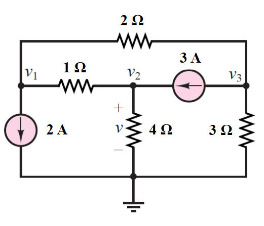
KCL at node :
KCL at node :
KCL at node :
From the node voltages, the power dissapated in the sources can be calculated. In the 2A source:
And in the 3A source:
Note that the voltage accross the current source is always calculated as the node the current is flowing to, minus the node the current is flowing from, ie (to - from). This makes the sign correct so it is known whether the source is delivering or absorbing power. If the direction of the current source oppose the direction of the voltage rise, it will be absorbing power..
If correct, the total power delivered to the circuit will equal the total dissapated. This calculation can be done to check, if you're bothered.
Dependant Sources
Some circuits contain current/voltage sources which are dependant upon other values in the circuit. In the example below, a current is assumed between the two nodes where the dependant voltage source is.
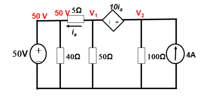
Calculate the power dissipated by the 50 resistor, and the power delivered by the current source.
At Node :
At Node :
We have two equations in 3 unknowns, so another equation is needed. Using :
These can be equated about to give
This system of equations solves to give , and .
Therefore,
- The power delivered by the current source
- The power dissapated by the 50 resistor is
Mesh Analysis
Achieves a similar thing to nodal analysis, using Kirchhoff's voltage law, and meshes instead of nodes.
Kirchhoff's Voltage Law
The sum of voltages around a closed loop always equals zero
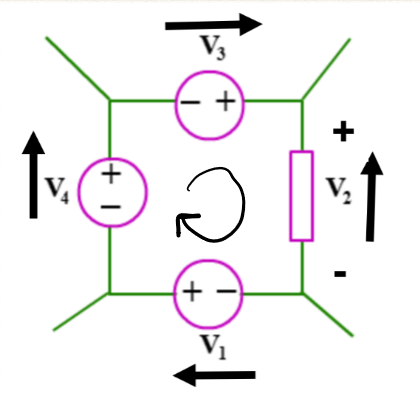
Sign convention
- If voltage rise and current in a voltage source are in the same direction, the voltage is denoted as negative
- If voltage rise and current are in opposite direction, voltage is positive
- In a resistor, current opposes voltage rise
Steps
- Identify meshes (loops) (always clockwise) and assign currents etc to those loops
- Apply KVL to each mesh to generate system of equations
- Solve equations
Where there are elements that are part of multiple meshes, subtract the currents of the other meshes from the mesh currently being considered to consider the total current through that circuit element.
Example
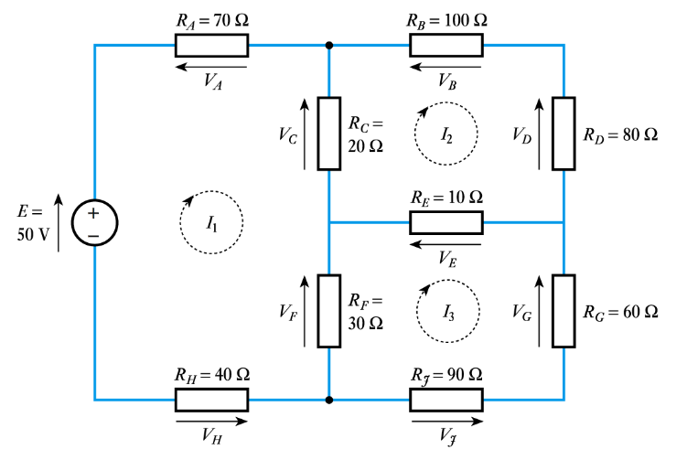
There are three meshes in this circuit, labelled , , .
For :
For :
For :
This forms a system of equations:
Solving yields , , and .
Impedance Matrices
Similar to how systems of equations from nodal analysis form admittance matrices, mesh analysis forms impedance matrices which describe the circuit being analysed. The matrix equation takes the form . As an example, the matrix equation for the system above is:
Therefore, the impedance matrix for the system is:
Another Example
Determine the currents in the circuit shown below:
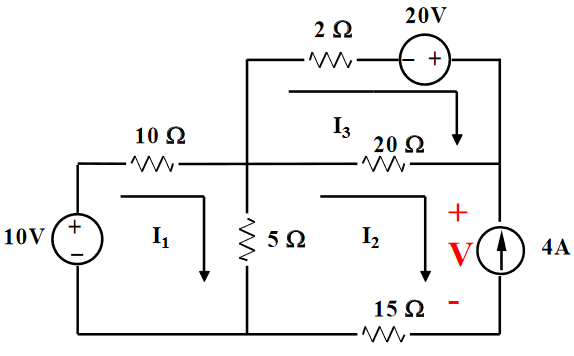
Loop 1:
Loop 2:
Where there is a current source, a voltage is assumed accross it.
Loop 3:
There are now 3 equations with 4 unknowns. However, it can be seen from the diagram that (the direction of the current source opposes our clockwise current), so the system can be solved as follows:
Example with dependant sources
Calculate the power dissapated in the 4 resistor and the power delivered/absorbed by the current dependant voltage source.
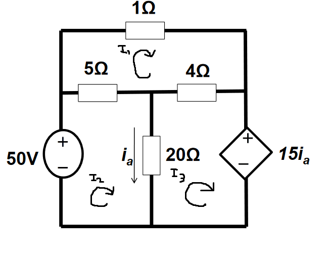
KVL round :
KVL round :
KVL round :
, so this can be substituted into equation 3 to obtain a fourth equation:
The system of equations then solves:
The power dissapated in the 4 resistor:
The power delivered/absorbed by the dependant voltage source: The source is absorbing power as the current opposes the direction of voltage rise in the source.
Thevenin and Norton Equivalent Circuits
Thevenin's Theorem states that as far as its appearance from outside is concerned, any two terminal network of resistors and energy sources can be replaced by a series combination of an ideal voltage source V and a resistor R, where V is the open-circuit voltage of the network and R is the resistance that would be measured between the output terminals if the energy sources were removed and replaced by their internal resistance.
In practice, this can be used for reducing complex circuits to a more simple model: taking networks of resistors/impedances and reducing them to a simple circuit of one source and one resistance.
- Thevenin circuits contain a single voltage source and resistor in series
- Norton circuits contain a single current source and a resistor in parallel
Calculating Equivalent Circuits
Any linear network viewed through 2 terminals is replaced with an equivalent single voltage & resistor.
- The equivalent voltage is equal to the open circuit voltage between the two terminals (/)
- The equivalent resistance () is found by replacing all sources with their internal impedances and then calculating the impedance of the network, as seen by the two terminals.
- This can be done alternatively by calculating the short circuit current (/) between the two terminals, and then using ohms law: .
- The value of the voltage source in a Thevenin circuit is
- The value of the current source in a Norton circuit is
- The value of the resistor in either circuit is
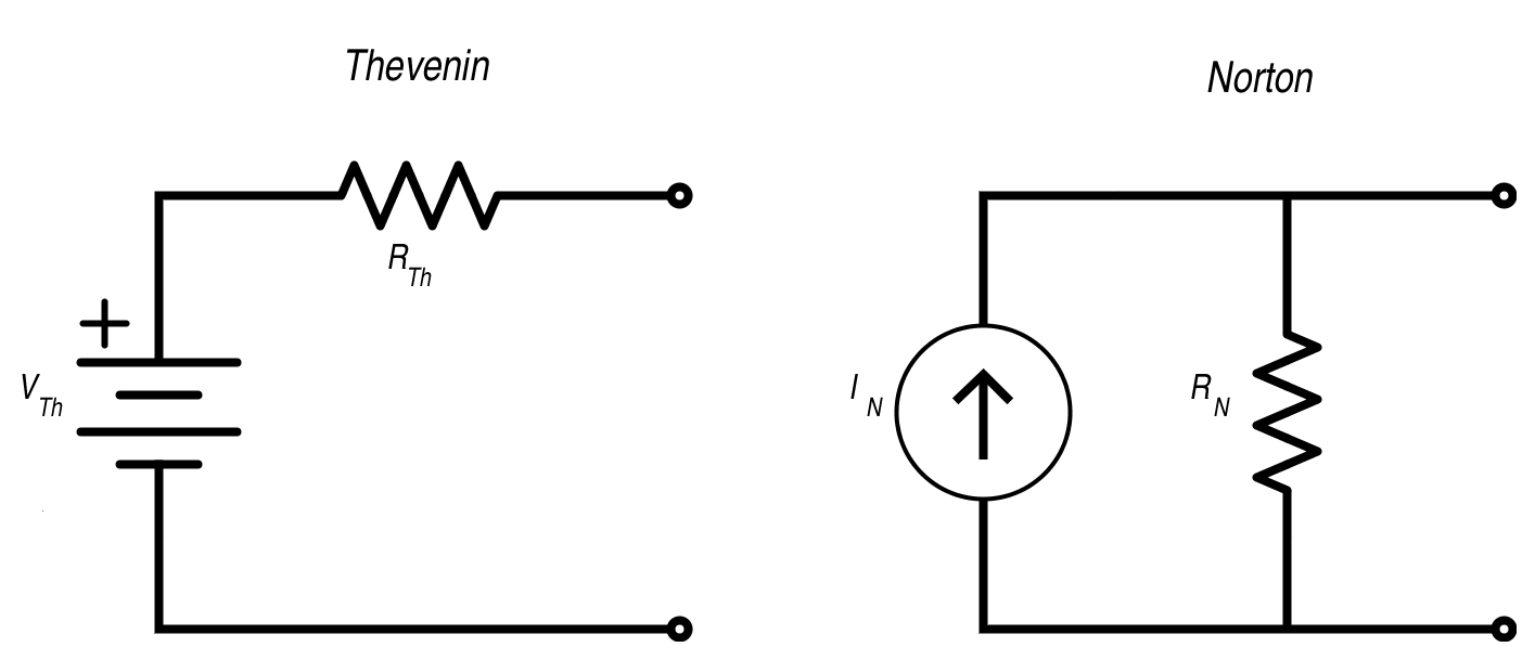
Often, nodal/mesh analysis is needed to determine the open circuit voltage and/or short circuit current.
Maximum Power Transfer
For the maximum power transfer between a source and a load resistance in a Thevenin circuit, the load resistance must be _equal to the thevenin resistance _. This can be trivially proved, and is left as an exercise to the reader.
Example 1
Determine the Thevenin equivalent of the following:
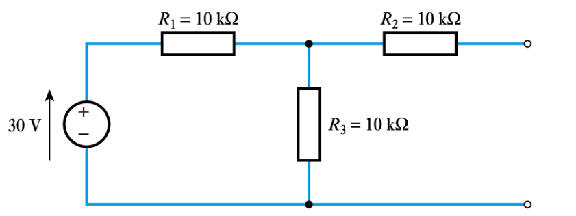
The open circuit voltage accross the two terminals can be calculated using the voltage divider rule, as the two resistors and split the voltage.
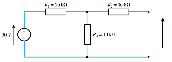
The short circuit current can be calculated by nodal analysis. When calculating the short circuit current, it is assumed that the two terminals are connected (shorted), so current can flow between them.
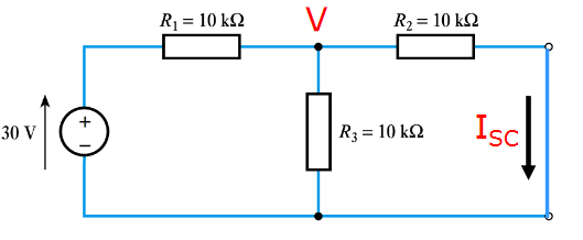
KCL at the node labelled V:
The voltage when the terminals are shorted is 10 V, so the short circuit current can be calculated using ohm's law:
Which gives
The resistance can alternatively be calculated by replacing the voltage source with it's internal resistance (0), and then determining the overall resistance of the network:
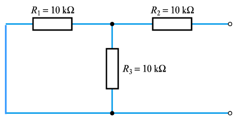
The resulting Thevenin circuit is therefore:
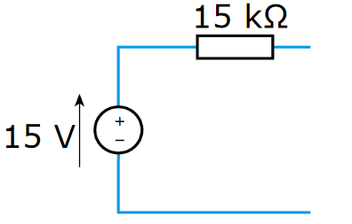
Example 2
Find the Thevenin equivalent circuit of the the network as seen by the two terminals A & B, and therefore the power dissapated/absorbed by the 12V source.
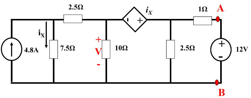
Open Circuit
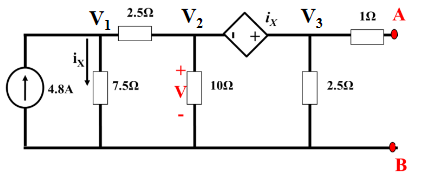
Doing nodal analysis to determine voltages:
: : :
Combining 2 & 3 by cancelling the assumed current :
Using to generate another equation:
This gives a system of 3 equations in 3 unknowns which can be solved to determine the node voltages:
is equal to , so
Short Circuit
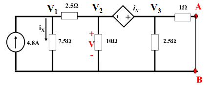
The same nodal analysis is needed, except this time the terminals are shorted. The steps are pretty much identical.
is the exact same,
: :
2 & 3 are combined in the same way, except yielding a slightly different equation, as this time current can flow to ground from through the 1 \Omega Resistor.
The third equation generated using is also the same,
The solution to this system is very similar to above:
The short circuit current is then calculated as:
Solution
The Thevenin resistance is calculated as:
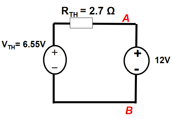
The power delivered to the 12V source is therefore:
First Order RC Circuits
RC circuits are those containing resistors and capacitors. First order means they can be modelled by first order differential equations
Capacitors
Capacitors are reactive elements in circuits that store charge. They work by creating an electric field between two parallel plates seperated by a dielectric insulator.
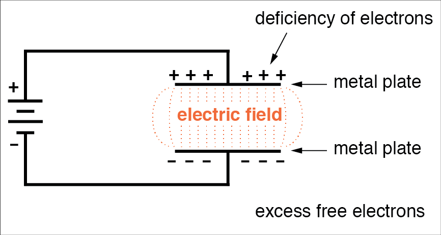
- When charging, the electrons between the plates separate. At full charge, all electrons will be on opposite plates.
- When discharging, the plates discharge and the charges recombine, forming a current
Equations
Capacitance of a specific capacitor, where
- = the area of the two plates
- = the separation of the two plates
- = the relative electric permittivity of the insulator
- = the permittivity of free space
The charge on a capacitor is equal to the product of the capacitance and the voltage accross it:
This can be used to derive the i-v equation for a capacitor:
This equation is important as it shows how current leads voltage in a capacitor by a phase of rads.
Energy
The energy stored in a capacitor:
Series and Parallel Combinations
Capacitance combines in series and parallel in the opposite way to resistors.
For capacitors in series:
In parallel:
Charging and Discharging
- When a voltage is applied to a capacitor, an electric field is formed between the two plates, and the dielectric becomes polarised.
- As the capacitor charges, the charges in the dielectric separate which forms a displacement current. At time , the capacitor behaves as a short circuit
- Capacitors charge exponentially, so the time at which one is fully charged is describes as time . At this time, the capacitor can take no more charge, so it behaves as an open circuit
- When discharging, the displaced charges flow round the circuit back to the other side of the capacitor.
- The charge decays exponentially over time.
Step Response
Capacitors charge and discharge at exponential rates, and there are equations which describe this response to a step input.
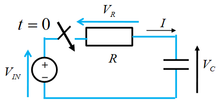
The step response of a charging capacitor at time , assuming the switch is closed at time :
Equations for current can be derived from this by differentiation:
Assuming , the equations for current and voltage when charging at time are:
Where and are the input current and voltage, respectively. Similar equations exist for discharging. Voltage at time when discharging:
Time constant
is the time constant of the circuit, which describes the rate at which it charges/discharges. 1 time constant is the time in seconds for which it takes the charge of a capacitor to rise by a factor of (approx 63%). As charging and discharging are exponential, a capacitor will only be fully charged when . However, in practical terms, a capacitor can be considered charged at .
Example
In the circuit below, determine equations for the response of the capacitor when the switch is moved to position 2.
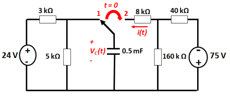
is equal to the voltage accross the capacitor at time , which is the same as the voltage accross the 5 resistor. When capacitors are fully charged, they are open circuit, so it is not conducing current, making the two voltages equal.
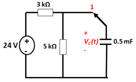
is equal to the voltage of the charging circuit as seen by the capacitor. This can be calculated as the thevenin equivalent of the circuit when the switch is in the right position.
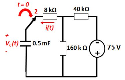
The time constant of the circuit:
Therefore:
The current can be calculated using :
Another Example
For the circuit shown below:
- Determine Thevenin circuit as seen by capacitor in position 1
- Calculate the time constant of the circuit for time
- Derive an equation for for
- Calculate the time taken for the capacitor voltage to fall to zero
- Derive an equation for for
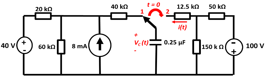
t < 0
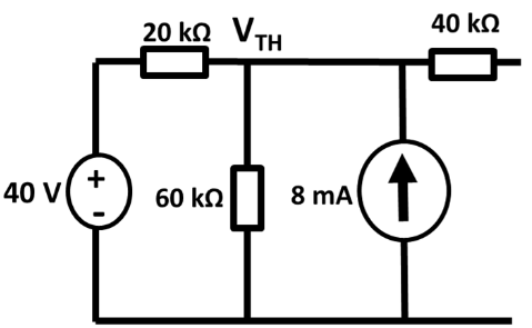
The Thevenin voltage of the left hand bit of the circuit can be calculated by KCL:
Calculating Thevenin resistance by summing resistances:
t > 0
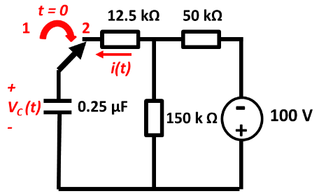
The Thevenin voltage of the right hand side as seen by the capacitor, using the voltage divider rule:
Thevenin Resistance:
This gives the time constant
Deriving transient equations:
For to fall to zero:
First Order RL Circuits
Basically the same as RC circuits, but with inductors instead.
Inductors
Inductors are reactive components, similar to capacitors. The difference is that while capacitors store energy in electric fields, inductors store it in magnetic fields. They do this with coils of wire wrapped around ferromangetic cores. Inductance is measured in Henries H and has symbol .
Inductance can be calculated as where
- is the number of turns in the coil
- is the circumference of the core
- is the cross-sectional area of the core
- is the permeability of free space
- is the relative permeability of the core
Inductance
-
Current passing through a conductor (the coil of wire) causes a change in magnetic flux which magnetises the coil.
-
This change in flux induces an EMF (Electro-Motive Force) in any conductor within it.
-
Faraday's Law states that the magnitude of the EMF induced in a circuit is proportional to the rate of change of flux linking the circuit
-
Lenz's Law states that the direction of the EMF is such that it tends to produce a current that opposes the change of flux responsible for inducing the EMF in the first place
-
Therefore, as we attempt to magnetise an inductor with a current, it induced a back EMF while it's field charges
-
One the inductor is fully charged, the back EMF dissapears and the inductor becomes a short circuit (it is just a coil of wire, after all).
-
When a circuit forms a single coil, the EMF induced is given by the rate of change of the flux
-
When a circuit contains many coils of wire, the resulting EMF is the sum of those produced by each loop
-
If a coil contains N loops, the induced voltage is given by the following equation, where is the flux of the circuit.
-
This property, where an EMF is induced by a changing flux, is known as inductance.
Self - Inductance
- A changing current causes a changing field
- which then induced an EMF in any conductors in that field
- When any current in a coil changes, it induced an EMF in the coil
This equation describes the I-V relationship for an inductor. It can be derived from the equations for faraday's law and inductance.
Energy Stored
The energy stored in an inductor is given by
Series & Parallel Combinations
Inductors sum exactly the same way as resistors do. In series:
And in parallel:
DC Conditions
The final constant values of a circuit, where current and voltage are both in a "steady-state" is known as DC conditions. Under DC conditions:
- Capacitor acts as open circuit
- Inductor acts as short circuit
Response of RL Circuits
Inductors exhibit the same exponential behaviour as capacitors. In a simple first order RL circuit:
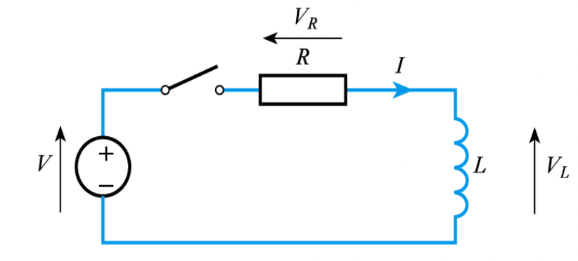
- Inductor is initially uncharged with a current at 0
- When the circuit is switched on at time t=0, is initially 0 as the inductor is open circuit.
- is initially 0
- is initially V
- As the inductor energises, increases, increases, so decreases
- This is where the exponential behaviour comes from
Equations for Step Response
Consider the circuit above, where thw switch is closed at time t=0. KVL can be used to derive an equation for the current in the circuit over time, which is shown below:
Where the time constant . The inductor voltage at time is equal to:
When discharging, the current at time is equal to:
Note that is equal to current / , by ohm's law.
RC vs RL Circuits
RC circuits and RL circuits are similar in some respects, but different in others.
RC Equations
RL Equations
Examples
In the circuit below, the switch is opened at time . Find:
- for
- for
- for
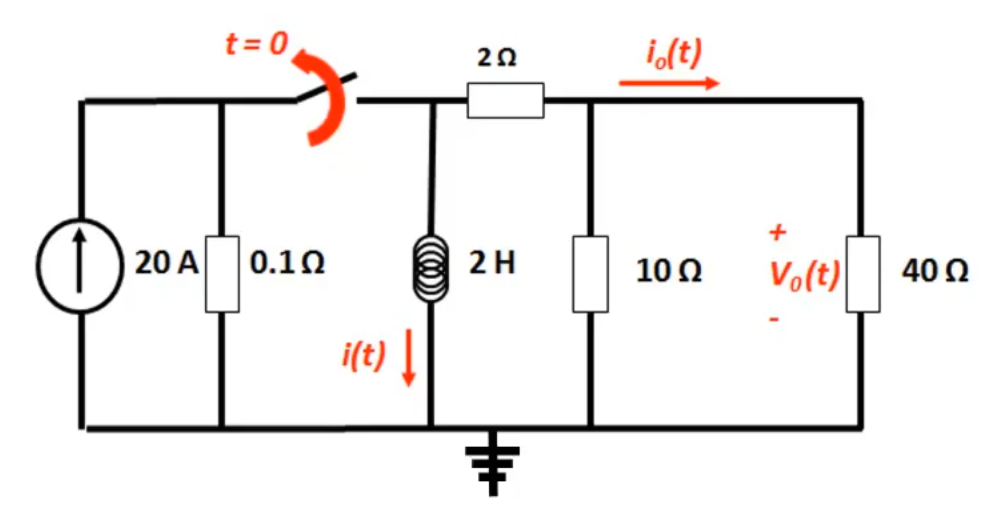
Looking for something of the form
In steady state, before the switch is opened, all of the current flows through the inductor as it is short circuit, meaning .
When the switch is opened there is no energy supplied to the circuit, so the inductor discharges through the right hand half of the circuit. The inductor can see a resistance of :
There is no input voltage, so:
This can simply be calculated using the current divider rule:
Using ohm's law:
AC Circuits
- AC current is the dominant form of electricity
- Current changes direction at a fixed frequency (usually 50~60Hz)
- AC voltage is generated by a rotating electromagnetic field
- The angular velocity of this rotation determines the frequency of the current
An instantaneous voltage in a sine wave is described by:
Where:
- is the peak voltage
- is the angular frequency (rad/s)
- is the phase shift (radians)
- The period of the wave is given by
, and define a waveform
As current and voltage are proportional, AC current is defined in a similar way:
Euler's Identity and Phasors
A phasor is a vector that describes a point in a waveform. A vector has a magnitude and a direction, which describe the amplitude and the phase of the signal, respectively. The rate at which the phasor "rotates" is the frequency of the signal.
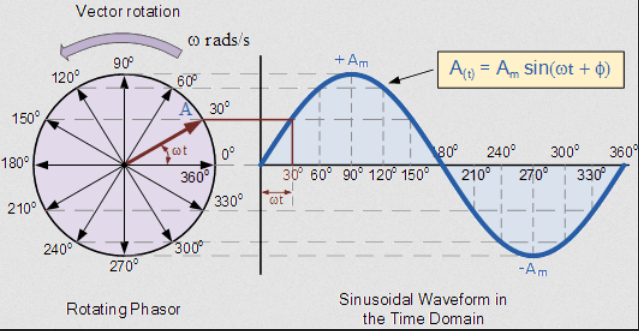
An AC phasor can be represented as a complex number.
This formula can be used to go from anywhere on a waveform to a phasor, for example:
Reactance and Impedance
- The ratio of voltage to current is a measure of how a component opposes the flow of electricity
- In a resistor, this is resistance
- In inductors and capacitors, this property is reactance, , measure in ohms
- Can still be used in a similar way to resistance
- Ohm's law still applies,
- Capacitative reactance
- Inductive reactance
- is the angular frequency of the AC current
- Both reactance and resistance are impedances
- Impedance is also measured in ohms
- The impedance of a component is how hard it is for current to flow through it
- Impedance represents not only the magnitude of the current, but the phase
Inductance
The voltage accross an inductor is:
In an AC circuit:
When an AC current flows through an inductor, an impedance applies
The impedance of an inductor is times its reactance:
Capacitance
Capacitors have a similar property:
Capacitive Impedance:
Complex Impedance
Impedance not only changes the magnitude of an AC current, it also changes its phase.
- In a capacitor, voltage leads current by a phase of 90 degrees
- In an inductor, current leads voltage by a phase of 90 degrees
- CIVIL: Capacitor I leads V, V leads I in inductor
The diagram below shows the effect of reactance on phase shift.
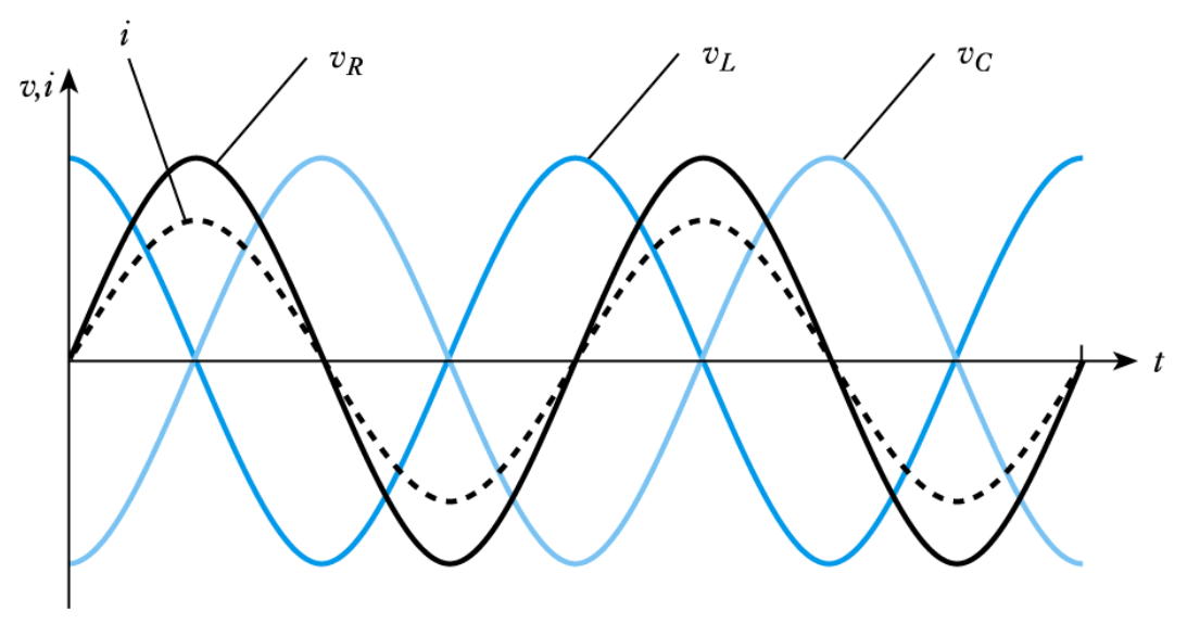
Consider the circuit below, containing an inductor and resistor in series. The phasor diagram shows the effect of the impedances on the voltage. The inductor introduces a phase shift of 90 degrees into the voltage.
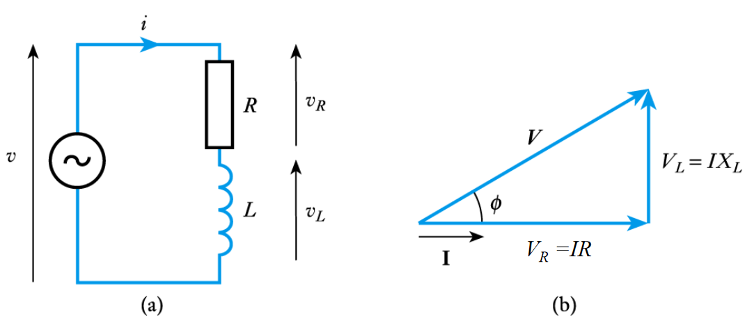
The magnitude of the voltage accross both components is: where Z is the magnitude of the impedance,
From the phasor diagram, the phase shift of the impedance is:
Complex impedances sum in series and parallel in the exact same way as normal resistance.
Example 1
Determine the complex impedance of the following combination at 50 Hz
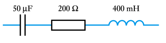
At 50Hz, the angular frequency rad/s
Example 2
Determine the complex impedance and therefore the current in the following combination
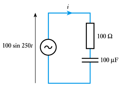
Since ,
The current can be calculated from the impedance using ohm's law:
Diodes
Diodes are semiconductor devices that allow current to flow only in one direction. Diodes look like this:
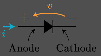
The diagram is labelled with an anode and a cathode. The voltage drop accross the diode is from anode -> cathode, and the current is conducted in the direction pointed by the really big black arrow.
The type's of diode's we're concerned with are silicon diodes, which have a forward voltage of about 0.7V. This is only an approximation, but is the value to use in calculations.
IV characteristics
Diodes are non-linear components:
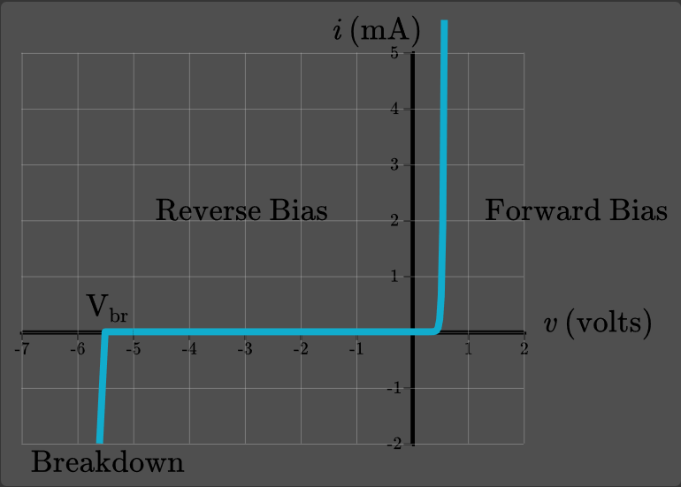
- When current is flowing from anode to cathode, the diode is forward-biased, and will conduct current
- When the current is flowing backwards (the wrong way), the diode is reverse-biased.
- At a large negative voltage, the diode will break down, and start to conduct current again
- Don't let the voltage get this high, you wont like what happens.
Forward Voltage
For the diode to conduct, it must have a minimum voltage accross it, known as the forward voltage. This is also always the total voltage drop accross the diode. For a silicon diode, this is 0.7V, which is why the I-V graph does not go up from zero. The diode can be said to "open" or "switch on" at about this voltage.
- If there is a voltage of 0.2V accross a diode, no current will flow
- If there is a voltage of 0.6V accross a diode, a tiny amount of current may flow
- At >0.7V, the full current will flow with no resistance.
Example 1
Find the current and the voltages accross each component in the circuit below.
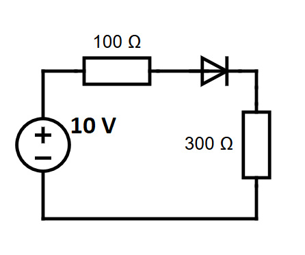
By Ohm's law, the current is:
Thefore, the voltages are
Example 2
Find the current through each resistor in the circuit below.
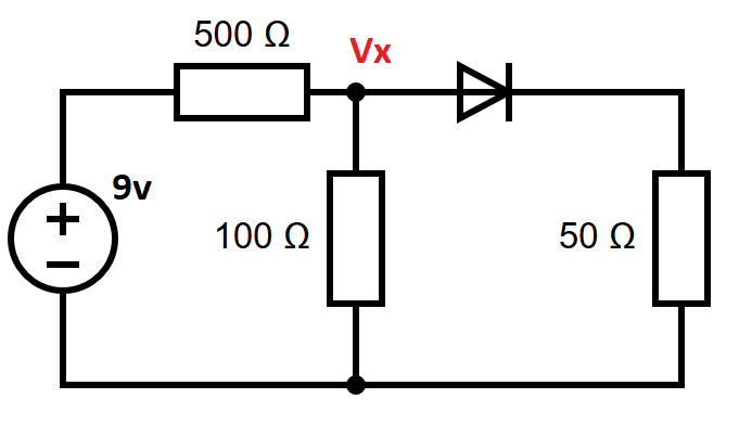
Doing KCL around node :
The three currents are then:
Transistors
Transistors are semiconductor devices based on P-N junctions. They have three terminals, the arrangement of which depends on the kind of transistor:
- Base
- Emitter
- Collector
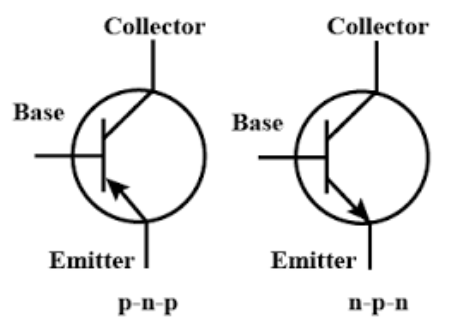
KCL applies, meaning the currents in the transistor sum to zero:
Transistors, like diodes are also semiconductors, meaning there is a voltage drop of 0.7 volts between the base and the emitter. When there is no collector current, transistors behave like a diode.
Transistors also have a current gain, meaning the current flowing into the collector is related to the current flowing into the base:
NPN Transistors
- The base-emitter junction behaves like a diode
- A base current only flows when the voltage is sufficiently positive, ie .
- The small base current controls the larger collector current, flowing from collector to emitter
- - the current gain, showing how base current controlls collector current
Functionally, transistors are switches that emit a current from collector to emitter dependant upon the base current.
Example
For the circuit below, find the base and collector currents using a gain of .
![]()
The base current can be calculated using ohm's law, taking into account the 0.7V drop between base and emitter:
As there is sufficient voltage for the transistor to be on, the collector current is therefore:
PNP Transistors
The diagram at the top of the page shows the circuit symbols for both kinds of transistor. The difference between the two is the way the emitter points, which is the direction of current flow in the transistor, and also the direction of voltage drop. An NPN transistor has a forward-biased junction, whereas PNP is reverse biased. Functionally, the difference between the two is that for a PNP transistor to be "on", the emitter should be at higher than the base.
Example
Note that this circuit uses a PNP transistor, so the base is at a lower voltage than the emitter. Also note that one of the resistors is not labelled. This is because the value of it is irrelevant, as the collector current is dependant upon the bias of the transistor.
![]()
Emitter Current
Notice that in the two examples, the collector current is much larger than the base, due to the large gain on the transistor. When there is a large gain :
From the example above:
Op Amps
Operational Amplifiers (Op-Amps) are high-gain electronic voltage amplifiers. They have two inputs, an output, and two power supply inputs. Op amps require external power, but this is implicit so is often emitted in circuit diagrams.
Op amps are differential amplifiers, meaning they output an amplified signal that is proportional to the difference of the two inputs. They have a very high gain, in the range of to , but this is assumed to be infinite in ideal amplifiers. The output voltage is calculated by:
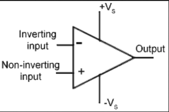
Ideal Model
An ideal model of an op amp is shown below
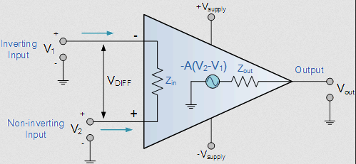
- Open loop gain is infinite
- The gain of the op amp when there is no positive or negative feedback
- Input impedance () is infinite
- Ideally, no current flows into the amplifier
- Output impedance () is zero
- The output is assumed to act like a perfect voltage source to supply as much current as possible
- Bandwith is infinite
- An ideal op amp can amplify any input frequency signal
- Offset Voltage is zero
- The output will be zero when the input and output voltage are the same
Ideal Circuits
Op amps can be used to design inverting and non-inverting circuits.
Inverting
- Negative feedback is used to create an amplifier that is stable, ie doesn't produce a massive voltage output.
- This creates closed loop gain, which controls the output of the amplifier
- The non-inverting input is grounded
- The negative feedback reverses the polarity of the output voltage
- As the output of the op amp is only a few volts, and the gain of the op amp is very high, it can be assumed that the voltage at both inputs is equal to zero volts
- This creates a "virtual earth" at the node shown on the diagram

Using KCL at this node, it can be shown that:
The gain of the amplifier is set by the ratio of the two resistors.
Non-Inverting
Non-inverting amplifiers don't invert the voltage output, and use input at the non-inverting terminal of the op amp instead.
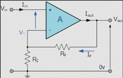
The output of the amplifier is calculated by:
Op Amps as Filters
Filters take AC signals as input, and amplify/attenuate them based upon their frequency.
Low Pass Filter
Take a simple inverting amplifier circuit, and add a capacitor in parallel.
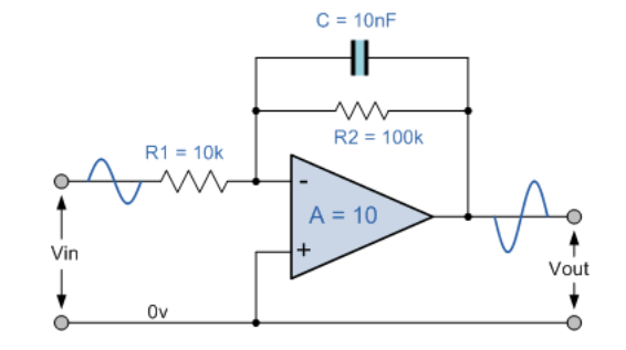
The gain is now a function of the input frequency, which makes the circuit a filter. The reactance of the capacitor . The impedance of the capacitor and resistor in parallel:
The gain as a function of is therefore:
- Gain is measured in decibels
- As the input frequency increases, gain decreases
- At very low frequencies, the gain is constant (0dB)
- The capacitor has high reactance at low frequencies, and is open circuit at very low frequencies
- At very high frequencies, the gain tends towards dB
- The capacitor has a very low reactance at high frequencies (short circuit)
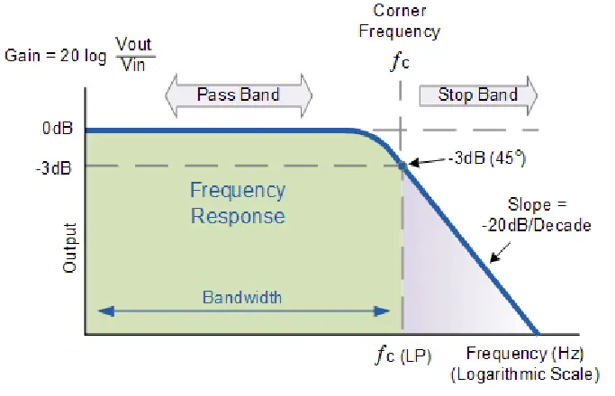
Cutoff Frequency
The cutoff frequency of a filter is the point at which the gain is equal to -3 dB, which corresponds to a fall in output by a factor of . For the filter shown above, this is:
High Pass Filter
A high pass filter is designed in a similar way
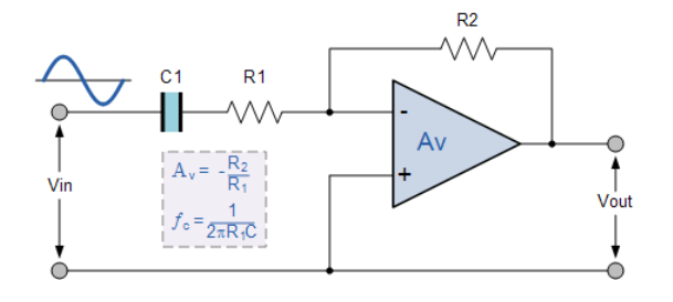
This time, the impedance of the capacitor-resistor combination is:
Which makes the gain:
The cutoff frequency for this filter is:
Which is similar to the other one, just with the other resistor.
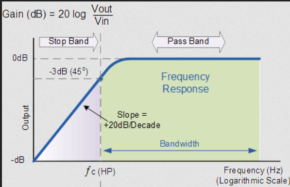
Voltage Transfer Characteristics
- The voltage transfer characteristic of an amplifier shows the output voltage as a function of the input voltage
- The output range is equal to the range of the power supplies
- Where the slope = 0, the amplifier is saturated
- Where the slope > 0, the gain is positive
- Where the slope < 0, the gain is negative
- When the amplifier is saturated the signal becomes distorted
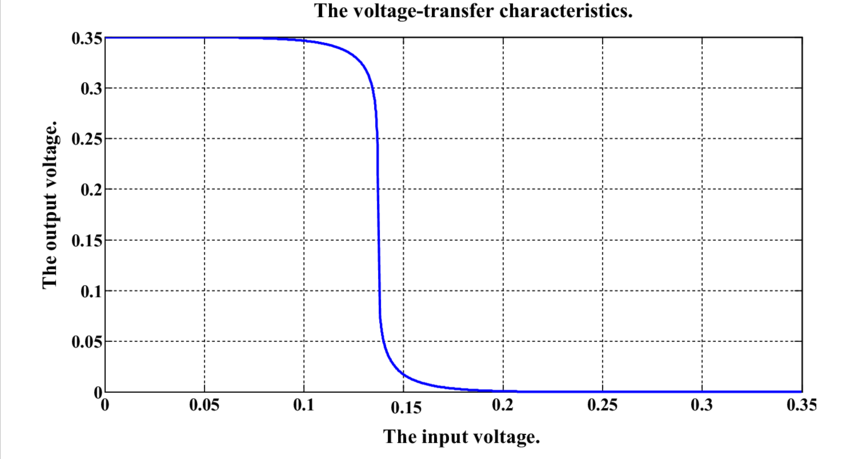
Passive Filters
Op amps are active filters because they require power. Passive filters use passive components (Resistors, Inductors, Capacitors) to achieve a similar effect. They are constructed using a potential divider with reactive components. The diagram below shows a potential divider with two impedances, and :
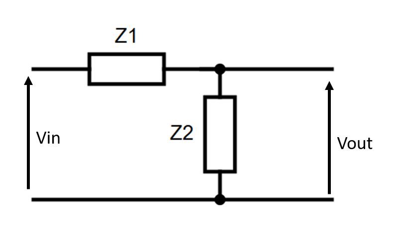
Transfer Functions
The transfer function is the ratio of input to output (see ES197 - Transfer Functions for more details.). For a passive filter, this is the ratio of output voltage to input voltage, as shown above. For a filter, this will be a function of the input waveform, . When and are both identical resistors :
However, if was a capacitor , :
The gain and phase of the output are then the magnitude and argument of the transfer function, respectively:
Cutoff Frequency
Similar to active filters, passive filters also have a cutoff frequency . This is the point at which the power output of the circuit falls by , or the output gain falls by -3dB, a factor of . Using the above example again (a low pass RC filter):
This is also the point at which
The filter bandwith is the range of frequencies that get through the filter. This bandwith is 0 to for low pass filters, or and upwards for high pass.
RC High Pass
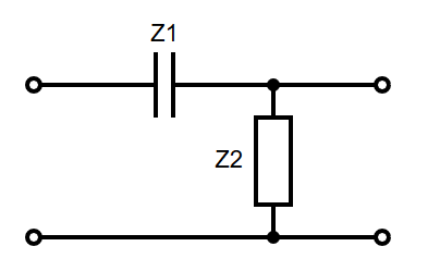
RC Low Pass
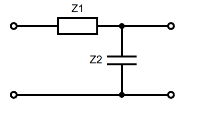
RL High Pass
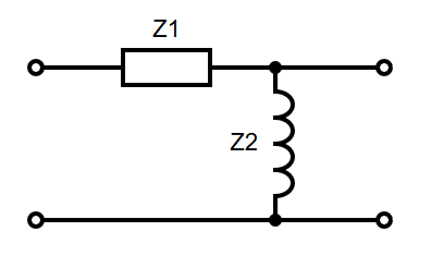
RL Low Pass
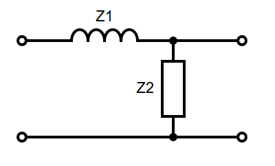
2nd Order Circuits
For circuits more complex than those above, to find the transfer function, either:
- Find a thevenin equivalent circuit, as seen from the element
- Combine multiple elements into single impedances
Note that any of the above techniques only work for simple first order circuits.
Example
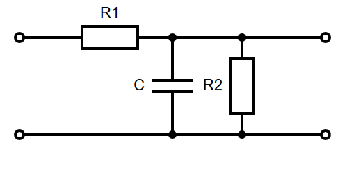
Using , where , and :
Equations
Below are some of the main equations that I have found useful to have on hand.
Capacitors
Energy Stored
The energy stored by a capacitor of capacitance, C with a voltage, v
- = Capacitance, Farads, F
- = Voltage, Volts, V
- = Charge, Coulombs, C
Capacitor Equation
The ratio of charge to voltage.
- = Capacitance, Farads, F
- = Voltage, Volts, V
- = Charge, Coulombs, C
Capacitance equation
- = the area of the two plates
- = the separation of the two plates
- = the relative electric permittivity of the insulator
- = the permittivity of free space
Series Capacitors
Parallel Capacitors
Current-Voltage
Step Response
- = Voltage of the capacitor at time t, Volts
- = Voltage in, Volts
- = Starting Voltage, Volts
- = Capacitance, Farads, F Derived from:
Electric Field Strength
- = Force
- = Charge
- = Permittivity of free space =
- = Constant
- = Voltage Potential, Volts
- = Separation
Capacitor Reactance
As the capacitor charges or discharges, a current flows through it which is restricted by the internal impedance of the capacitor. This internal impedance is commonly known as Capacitive Reactance
- = Reactance of the Capacitor, Ohmns
- = =
- = frequency, rads per second
Flux Density
The amount of flux passing through a defined area that is perpendicular to the direction of the flux.
Magnetic Field Strength of Straight Current Carrying Wire
Amperes Law: For any closed loop path, the sum of the products of the length elements and the magnetic field in the direction of the length elements is proportional to the electric current enclosed in the loop.
- = Magnetic field strength at distance d
- = Current
- = Permeability of free space =
- = distance from the wire.
Inductors
Inductors in Series
Inductors act in the same way as resistors in terms of their behaviour in series and parallel.
Inductors in Parallel
Induced Voltage
If a coil contains N loops, the induced voltage V is given by the following equation, where Φ is the flux of the circuit.
Self Inductance
A changing current causes a changing field, which then induced an EMF in any conductors in that field, When any current in a coil changes, it induced an EMF in the coil
Energy Stored
The energy stored by an inductor is given by:
Step Response of RL Circuit (Current)
- - Voltage source
- - Resistance of the resistor
- - The initial current. (If is already charged, then will be short circuit current)
Step Response of RL Circuit (Voltage)
Inductor voltage at time t,
- - Voltage across inductor at time t
- - Voltage source
- - Resistance of the resistor
- - The initial current
Thevenin and Norton Equivalent Circuits
Thevenin circuits contain a single voltage source and resistor in series. Norton circuits contain a single current source and a resistor in parallel
Equivalent Resistance
Any linear network viewed through 2 terminals is replaced with an equivalent single voltage & resistor.
- The equivalent voltage is equal to the open circuit voltage between the two terminals (/)
- The equivalent resistance () is found by replacing all sources with their internal impedances and then calculating the impedance of the network, as seen by the two terminals.
- This can be done alternatively by calculating the short circuit current (/) between the two terminals, and then using ohms law: .
- The value of the voltage source in a Thevenin circuit is
- The value of the current source in a Norton circuit is
- The value of the resistor in either circuit is
Thevenin - Norton Conversion
Thevenin and Norton are essentially the same, but in a different form. The is the same for both.
- - Norton Current
- - Thevevin Voltage
- - Thevenin Resistance
AC Circuits
- AC current is the dominant form of electricity,
- Current changes direction at a fixed frequency (usually 50~60Hz)
- AC voltage is generated by a rotating electromagnetic field
- The angular velocity of this rotation determines the frequency of the current
Instantaneous Voltage
An instantaneous voltage V in a sine wave is described by
Where:
- is the peak voltage
- is the angular frequency (rad/s)
- is the phase shift (radians)
- The period of the wave is given by
Instantaneous Current
As current and voltage are proportional, AC current is defined in a similar way:
AC Phasor - As complex number
An AC phasor can be represented as a complex number.
Operational Amplifiers
Output of Inverting Amplifier
The gain of the amplifier is set by the ratio of the two resistors. The negative feedback reverses the polarity of the output voltage (Hence Negative).
Output of Non-Inverting Amplifier
Non-inverting amplifiers don't invert the voltage output, and use input at the non-inverting terminal of the op amp instead.
Filters
Cutoff Frequncy
The cutoff frequency of a filter is the point at which the gain is equal to -3 dB, which corresponds to a fall in output by a factor of . For the filter shown above, this is:
Gain (dB)
Gain is measured in decibels
At very low frequencies, the gain is constant (0dB) The capacitor has high reactance at low frequencies, and is open circuit at very low frequencies At very high frequencies, the gain tends towards − dB The capacitor has a very low reactance at high frequencies (short circuit)
ES193
Functions, Conics & Asymptotes
Domain & Range
- The domain of a function is the set of all valid/possible input values
- The x axis
- The range of a function is the set of all possible output values
- The y axis
Odd & Even Functions
Conics
Equation of a circle with radius and centre
Equation of an ellipse with centre , major axis length and minor axis length :
Equation of a Hyperbola with vertex :
The asymptotes of this hyperbola are at:
Asymptotes
There are 3 kinds of asymptotes:
- Vertical
- Horizontal
- Oblique (have slope)
For a function :
- Vertical asymptotes lie where and
- Horizontal asymptotes
- If the degree of the denominator is bigger than the degree of the numerator, the horizontal asymptote is the x-axis
- If the degree of the numerator is bigger than the degree of the denominator, there is no horizontal asymptote.
- If the degrees of the numerator and denominator are the same, the horizontal asymptote equals the leading coefficient of the numerator divided by the leading coefficient of the denominator
- Oblique asymptotes
- A rational function will approach an oblique asymptote if the degree of the numerator is one order higher than the order of the denominator
- To find
- Divide by
- Take the limit as
Example: find the asymptotes of :
- Vertical asymptotes:
- Where the denominator is 0
- Horizontal asymptotes:
- There are none, as degree of the numerator is bigger than the degree of the denominator
- Oblique asymptotes:
- Divide the top by the bottom using polynomial long division
- Find the limit
As , , giving as an asymptote.
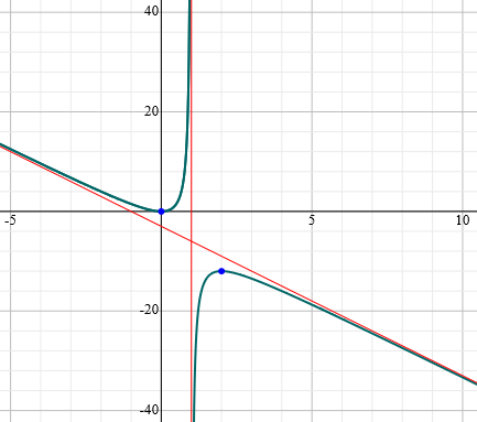
Complex Numbers
De Moivre's Theorem
Complex Roots
For a complex number
The roots can be found using the formula
Finding Trig Identities
Trig identities can be found by equating complex numbers and using de moivre's theorem. The examples below are shown for n=2 but the process is the same for any n.
Identities for
Using de moivre's theorem to equate
Expanding
Equating real and imaginary parts
Identities for
To find the identity for , start with , and raise to the power of 2
Substituting in for the pairs of
Vectors
Vector Equation of a Straight Line
The vector is the vector of any point along the line.
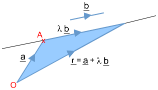
is any point on the line, and \bm{b} is the direction of the line. is a parameter that represents the position of relative to along the line. The carteian form of this can be derived:
Equating about lambda:
Scalar/Dot Product
The dot product of two vectors:
- If , then and
- The two vectors are perpendicular
The angle between two vectors can be calculated using the dot product
Projections
The projection of vector in the direction of is given by the scalar product:
This gives a vector in the direction of with the magnitude of .
Equation of a Plane
The vector equation of a plane is given by
Where is the normal to the plane, and is any point in the plane. This expands to the cartesian form:
Angle Between Planes
The angle between two planes is given by the angle between their normals.
Intersection of 2 Planes
Two planes will only intersect if their normal vectors intersect.
- First, check the two normals are non parallel
- Equate all 3 variables about either a parameter or one of , , or to get an equation for the line along which the planes intersect in cartesian form
Example
Find the intersection of the planes (1) and (2).
(1) - (2):
(1) + 3(2):
Equating the two with z:
Using Cross Product
For two normals to planes and , the vector will lie in both planes. The line
lies in both planes.
Distance from Point to Plane
The shortest distance from the point to the plane is given by:
Vector/Cross Product
The cross product of two vectors produces another vector, and is defined as follows
is the angle between the two vectors, and is a unit vector perpendicular to both and . The right-hand rule convention dictates that should always point up (ie, if and are your fingers, then is your thumb). The cross product is not commutative, as = .
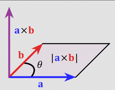
- The magnitude of the cross product is equal to the area of the parallelogram formed by the two vectors.
- Can be used to find a normal given 2 vectors/2 points in a plane
Angular Velocity
A spheroid rotates with angular velocity . A point on the spheroid has velocity
Matrices
Determinant & Inverse of a 2x2 Matrix
The determinant of a 2x2 matrix:
The inverse:
The inverse of a matrix only exists where
Minors & Cofactors
- There is a matrix minor corresponding to each element of a matrix
- The minor is calculated by
- ignoring the values on the current row and column
- calculate the determinant of the remaining 2x2 matrix
Example:
The minor of the top left corner is:
The cofactor is the minor multiplied by it's correct sign. The signs form a checkerboard pattern:
The matrix of cofactors is denoted .
Determinant of a 3x3 Matrix
The determinant of a 3x3 matrix is calculated by multiplying each element in one row/column by it's cofactor, then summing them. For the matrix:
This shows the expansion of the top row, but any column or row will produce the same result.
Inverse of a 3x3 Matrix
- Calculate matrix of minors
- Calculate matrix of cofactors
- Transpose
- Multiply by 1 over determinant
Example
The transposed matrix of cofactors is therefore:
Explanding by the bottom row to calculate the determinant (it has 2 zeros so easy calculation):
Calculating inverse:
Simultaneous Linear Equations
Several methods for solving systems of simultaneous linear equations. All the examples shown are for 3 variables, but can easily be expanded 2 variables.
Cramer's Rule
For a system of 3 equations:
- Calculate the determinant of the matrix of coefficients
- Calculate determinants by replacing 1 column of the matrix with the solutions
- Use determinants to calculate unknowns
Matrix Inversion
For a system of equations in matrix form The solutions is given by
The system has no solutions if
Gaussian Elimination
Eliminating variables from equations one at a time to give a solution. Generally speaking, for a system of 3 equations
First, eliminate x from and
This gives
Then, eliminate y from
Giving
This gives a solution for , which can then be back-substituted to find the solutions for and .
The advantages of this method are:
- No need for matrices (yay)
- Works for homogenous and inhomogeneous systems
- The matrix need not be square
- Works for any size of system if a solution exists
Sometimes, the solution can end up being in a parametric form, for example:
This doesn't make sense, as the final equation is satisfied for any value of . Substituting a parameter for gives:
Gauss-Seidel Iteration
Iterative methods involve starting with a guess, then making closer and closer approximations to the solution. If iterations tend towards a limit, then the system converges and the limit will be a solution. If the system diverges, there is no solution for this iteration. For the gauss-seidel scheme:
Rearrange to get iterative formulae:
Using these formulae, make a guess at a starting value and then continue to iterate. For example:
Rearranging:
The solutions are , , , as can be seen from the table below containing the iterations:
| r | x | y | z |
|---|---|---|---|
| 0 | 0 | 0 | 0 |
| 1 | 2.25 | 2.35 | 2.467 |
| 2 | 1.046 | 2.098 | 2.952 |
| 3 | 0.988 | 2.012 | 3.000 |
| 4 | 0.997 | 2.001 | 3.001 |
Note that this will only work if the system is diagonally dominant. For a system to be diagonally dominant, the divisor of the iterative equation must be greater than the sum of the other coefficients.
Systems can be rearranged to have this property:
Rearranges to:
Differentiation
Implicit Differentiation
When differentiating a function of one variable with respect to another (ie ), simply differentiate with respect to , then multiply by .
For example, find where . First, using the product rule to differentiate the first term:
The equation with all terms differentiated:
Rearranging to get in terms of :
Inverse Trig Functions
All the derivatives of the inverse trig functions are given in the data book. They can be derived as follows ( is used as an example).
Differentiating both sides with respect to x
Using pythagorean identity
Differentials
Differentials describe small changes to values/functions
Recall that . This means this can be rewritten:
Dividing both sides by :
represents a relative change in y, and represents a relative change in x. This can be used to give approximations of how one quantity changes based upon another.
For example, given the mass of a sphere , where is the material density, estimate the change in mass when the radius is increased by 2%.
Dividing both sides by the original formula:
represents a relative change in radius, so when increases by 2%,
Meaning the mass increases by 6%.
Hyperbolic Functions
Hyperbolic functions have similar identities to circular trig functions. They're the same, except anywhere there is a product of two s, the term should be negated. Hyperbolic functions can also be defined in terms of exponential functions, making them easy to differentiate.
All the derivatives of hyperbolic functions are given in the formula book.
Parametric Differentiation
For a function given in parametric form , :
Partial Differentiation
For a function of two variables there are two gradients at the point , one in and one in . To find the gradient in the x direction, differentiate treating y as a constant. To find the gradient in the y direction, differentiate treating x as a constant. These are the two partial derivatives of the function, and .
For example, for a function :
Implicit Partial Differentiation
When a function of several variables is given and a partial derivative is required, differentiate the numerator of the partial derivative implicitly with respect to the denominator, and treat the third variable as constant. For example, find given :
Another example, find given
Higher Order Partial Derivatives
Three 2nd order derivatives for functions of 2 variables. For :
Note how for the last one, the order is interchangable as it yields the same result.
Chain Rule
The chain rule for a function , where x and y are functions of a parameter :
Total Differential
The total differential represents the total height gain or lost when moving along the function described by
Contour Plots
Along a line of a contour plot, the total differential is zero: the height doesn't change. This allows to be found
Integration
Integration by Parts
When an integral is a product of two functions (ie ), it can be integrated by parts:
(see also the DI method)
Improper Integrals
An integral is improper if either
- One of its limits is infinity
- The function is not defined for any point within the interval (bounds inclusive)
To evaluate these integrals, replace the dodgy boundwith a variable , evaluate the integral in terms of the variable, and then take the limit as the variable tends towards the bound.
Where functions are not continuous over the interval, may need to split the function into two integrals. For example, if is not continuous at where , then:
Reduction Formulae
Reduction formulae involve rewriting an integral in terms of itself to get a recurrence relation. They usually involve some variable as well as other variables in the integral (). For example, integrating :
By parts:
Note how the integral is now in terms of itself, but with . This creates a recursive definition that can be expanded to evaluate
Integration by Substitution
Substitution is often useful in solving integrals.
- Choose a new function
- Find
- Substitute in
- Swap for
- Put limits in terms of (if appropriate)
- Solve with respect to u
Choosing a function to substitute depends on the integral, and there are certain patterns to spot which make it easier.
Example
Substituting :
Substituting the limits: The integral becomes:
Substitutions
There are two standard substitutions that can be really useful when integrating trig functions.
Subs
The first one:
For example:
Letting :
Subs
For example:
Letting :
Standard Forms
Integrals will sometimes be (or can be put into) standard forms which then evaluate directly to inverse trig functions. The full list is given in the data book but:
Example
Substituting
Trigonometric Identities
Trig identities are often useful in evaluating integrals, for example:
Using :
Integration as a Limit
The area under a curve from is given by: This can be approximated by dividing the area under the curve into a number of rectangles:
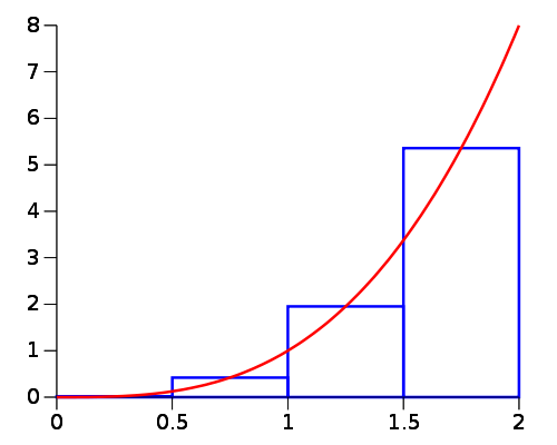
For rectangles over the width , the width of each rectangle . The area of the rectangle is therefore given by . The sum of all the rectangles, and therefore total area is:
As , , so:
Volumes of Revolution
For a function rotated 360 degrees about the x axis, consider a disc of width and radius y. The volume is given by . The volume of all slices as is
Therefore the volume of revolution for a function about the x axis is
Volume of revolution about y axis:
Centres of Mass for Planar Objects
The centre of mass is the point through which gravity acts. In 1 dimension:
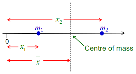
The sum of the moments about 0 is . The moment of the total mass is . Equating these:
This can be expanded into 2 dimensions:
For the centre of mass of an infinitely thin sheet with uniformly distributed mass, for x-axis consider thin slices of width .
- Area of slice =
- Mass of slice =
- Moment of slice about y-axis =
- Sum of all moments as =
For the sum of the moments about y axis, take a horizontal slice with width with length
- Area of slice =
- Mass of slice =
- Moments of slice about x-axis =
- Sum of all moments as =
Note that usually, mass is mass per unit area.
Example
Find centre of mass of plane lamina shown
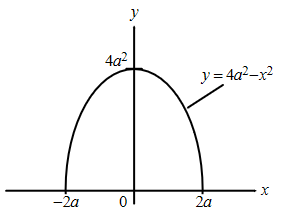
By symmetry, clearly . For , let be the mass per unit area, and consider a horizontal strip of width .
- Area of strip is
- Mass of strip is
- Moment of one strip about x axis is
Total moment as :
For the total mass , total area of the shape:
So total mass M =
Moments of Inertia for Laminae
The moment of inertia is a measure of how difficult it is to rotate an object. Suppose a lamina is divided into a large number of small elments, each with mass at distance from the origin . The moment of inertia of one element is defined to be . Taking the sum of all moments as
The bounds of the integral should be chosen appropriately such as to include the entire lamina.
- For a lamina lying in the x-y plane, the moment of inertia about z-axis is the sum of the moments about x and y axes.
- For an axis parallel to at a distance and both lying in the same plane as the lamina with mass , where passes through the centere of the lamina:
Example
Find the moment of inertia of a thin rectangular plate of mass , length and width about an axis through its centre of gravity which is normal to its plane.
Assuming the plate lies in the x-y axis, the question is asking for the moment about the z-axis. To find this, the moments about both x and y axes are required as . To find :
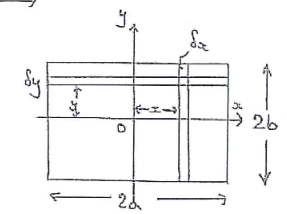
- Let the mass per unit area
- A strip of width at distance from has mass
- The moment of inertia of the strip is
Taking the limit of the sum of all the strips:
As ,
is identically dervied and equals . Summing the two moments gives:
Lengths of Curves
The length of the arc of a curve between and is given by
Alternatively, for parametrised curves:
Surface Areas of Revolution
Similar to volumes of revolution, the surface area of a function when rotated about the x axis is given by:
Example
The surface are of the parabola between and , when rotated about x axis:
Mean Values of a Function
For a function over the interval
Mean value:
Root mean square value:
Differential Equations
First Order
A first order differential equation has as it's highest derivative. For the two methods below, it is important the equation is in the correct form specified.
Seperating Variables
For an equation of the form
The solution is
Integrating Factors
For an equation of the form
An integrating factor can be found such that:
Multiplying through by gives
Then, applying he product rule backwards gives a solution:
Second Order
A second order ODE has the form:
The equation is homogeneous if .
The auxillary equation is
This gives two roots and , which determine the complementary function:
| Roots | Complementary Function |
|---|---|
| and both real | |
| , both real | |
| and |
The complementary function is the solution. Sometimes, initial conditions will be given which allow the constants and to be found.
Non-Homogeneous Systems
If the system is non-homogenous, ie , then a particular integral is needed too, and the solution will have form . The particular integral is found using a trial solution, then substituting it into the equation to find the coefficients. Note that if the particular integral takes the same form as the complementary function, an extra will need to be added to the particular integral for it to work, it would become
| Trial Solution | |
|---|---|
| const | const |
| polynomial | |
| or | |
Example
Auxillary equation:
Complementary function is therefore:
System is non-homogeneous, so have to find a particular integral. For this equation , so the p.i. is .
Substituting this into the original equation:
Comparing coefficients:
The general solution is therefore:
Using initial conditions to find constants, for
For
Particular solution for given initial conditions is therefore:
Laplace Transforms
The laplace transform transforms a function from the time domain to the laplace domain. For a continuous function . with , the laplace transform is defined as
The notation used is
Where is the function in the laplace domain. Tables of laplace transforms for common functions are given in the formula book, so there is no need to work out most transforms manually.
Transforms are linearly independent in the same way integrals are:
For example, find the laplace transform of :
Inverse Transforms
Transforms also have an inverse:
For example, find from
Sometimes, partial fractions and/or completing the square is required to get the equation into a form recognisable from the table.
First Shift Theorem
Differential Equations
Laplace transforms exist of derivatives:
This can be used to solved differential equations, by laplace transforming the differential equation to make an algebraic one, then inverse laplace transforming the result back.
Example
Solve:
Need to use partial fractions to inverse transform
Taking inverse laplace transforms using table:
Probability & Statistics
Probability
Set Theory
- A set is a collection of elements
- Elements are members of a set
- means "the element is a member of the set
- The empty set contains no elements
- It is empty
-
- is a set consisting of those integers
-
-
-
- is a subset of
- implies
- for all sets
- if and only if and
- is the union of and
- Set of elements belonging to or
- is the intersection of and
- Set of elements belonging to and
- Disjoint sets have no common elements
- is the different of and
- Set of elements belonging to but not
- is the complement of
- Set of elements not belonging to
Random Processes & Probability
The probability of event occurring is denoted . This is the relative frequency of event occurring in a random process within sample space S.
-
- Certain or sure event, guaranteed 100% to happen
-
- Impossible event, won't happen
-
- Elementary event, the only event that can happen, the only possible outcome
-
- Event that occurs if or occurs
-
- Event that occurs if and occur
-
- Event that occurs if does not occur
-
- Events and are mutually exclusive
Example
Toss a coin 3 times and observe the sequence of heads and tails.
- Sample space
- Event that heads occur in succession
- Event that 3 heads or 3 tails occur
Another Example
Sample space . Each number is an individual event.
| Events | Frequency | Relative Frequency |
|---|---|---|
| 17 | 3 | 3/35 |
| 18 | 4 | 4/35 |
| 19 | 9 | 9/35 |
| 20 | 11 | 11/35 |
| 21 | 6 | 6/35 |
| 22 | 2 | 2/35 |
Axioms & Laws of Probability
- for all
- Probabilities are always between 0 and 1 inclusive
-
- Probability of the certain event is 1
- If then
- If two events are disjoint, then the probability of either occurring is equal to the sum of their two probabilities
-
- The probability of the impossible event is zero
-
- The probability of all the elements not in A occurring is the opposite of the probability of all the elements in A occurring
- If , then
- The probability of A will always be less than or equal to the probability of B when A is a subset of B
-
- The probability of A minus B is equal to the probability of A minus the probability of A and B
-
- Probability of A or B is equal to probability of A plus the probability of B minus the probability of A and B
- This is important
Example
In a batch of 50 ball bearings:
- 15 have surface damage ()
- 12 have dents ()
- 6 both have defects ()
The probability a single ball bearing has surface damage or dents:
The probability a single ball bearing has surface damage but no dents:
Conditional Probability & Bayes' Theorem
A conditional probability is the probability of event occurring, given that the event has occurred.
Bayes' theorem:
Axioms of conditional probability:
Example
In a semiconductor manufacturing process:
- is the event that chips are contaminated
- is the event that the product containing the chip fails
- and
Determining the rate of failure:
Independent Events
Two events are independent when the probability of one occurring does not dependend on the occurrence of the other. An event is independent if and only if
Example
Using the coin flip example again with a sample space and 3 events
A and C are independent events:
B and C are not independent events:
Discrete Random Variables
For a random process with a discrete sample space , a discrete random variable is a function that assigns a real number to each outcome .
- is a measure related to the random distribution.
- Denoted
Consider a weighted coin where and . Tossing the coin twice gives a sample space , which makes the number of heads a random variable . Since successive coin tosses are independent events:
Events are also mutually exclusive, so:
This gives a probability distribution function of:
Cumulative Distribution Functions
The cumulative probability function gives a "running probability"
- if then
Using coin example again:
Expectation & Variance
- Expectation is the average value, ie the value most likely to come up
- The mean of
- Variance is a measure of the spread of the data
- Standard deviation
Using the weighted coin example once more:
Standardised Random Variable
The standardised random variable is a normalised version of the discrete random variable, obtained by the following transformation:
Binomial Distribution
- The binomial distribution models random processes consisting of repeated independent events
- Each event has only 2 outcomes, success or failure
The probability of successes in events:
- Probability of no success
- Probability of successes is
Expectation & Variance
Example
A fair coin is tossed 6 times.
Probability of exactly 2 heads out of 6
Probability of heads
Probability of heads
Expected value
Variance
Poisson Distribution
Models a random process consisting of repeated occurrence of a single event within a fixed interval. The probability of occurrences is given by
The poisson distribution can be used to approximate the binomial distribution with . This is only valid for large and small
Expectation & Variance
Example
The occurrence of typos on a page is modelled by a poisson distribution with .
The probability of 2 errors:
Continuous Random Variables
Continuous random variables map events from a sample space to an interval. Probabilities are written , where is the random variable. is defined with a continuous function, the probability density function.
- The function must be positive
- The total area under the curve of the function must be 1
Example
Require that , so have to find :
Calculating some probabilities:
Cumulative Distribution Function
The cumulative distribution function up to the point is given as
- if , then
-
- Derivative of cumulative distribution function is the probability distribution function
Using previous example, let . For
For
For
Expectation & Variance
Where is a continuous random variable:
Uniform Distribution
A continuous distribution with p.d.f:
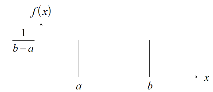
Expectation and variance:
Cumulative distribution function:
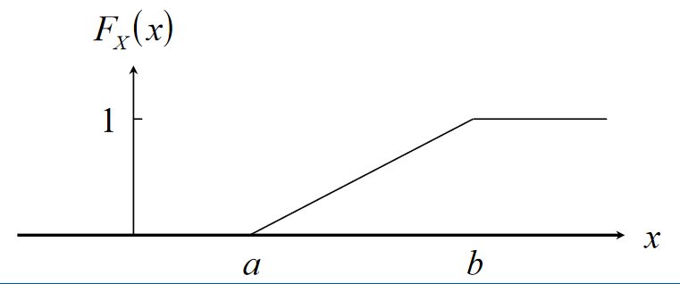
Exponential Distribution
A continuous distribution with p.d.f:
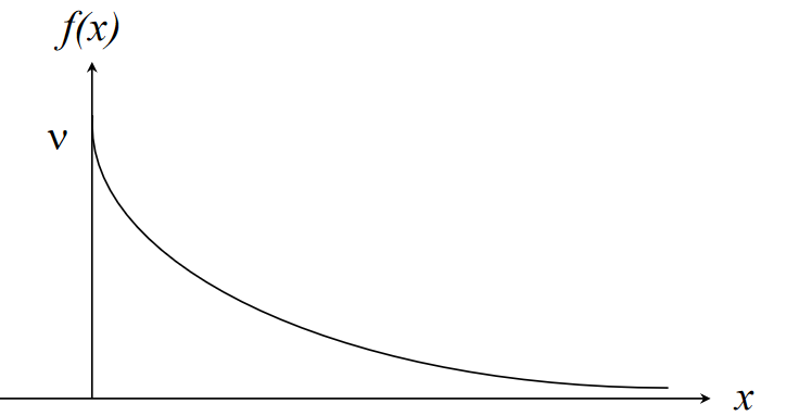
Expectation and variance:
Cumulative distribution function:
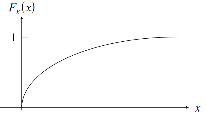
- Recall that a discrete random process where a single event occurs times in a fixed interval is modelled by a Possion distribution
- Consider a situation where the event occurs at a constant mean rate per unit time
- Let , then and probability of events occurring is
- Suppose the continuous random variable is the time between occurrences of successive events
- If there is a period of time with no events, then and
- If events occur then and
If the number of events per interval of time is Possion distributed, then the length of time between events is exponentially distributed
Example
Calls arrive randomly at the telephone exchange at a mean rate of 2 calls per minute. The number of calls per minute is a d.r.v. which can be modelled by a Poisson distribution with . The probability of 1 call in any given minute is:
The time between consecutive calls is a c.r.v. modelled by an exponential distribution with . The probability of at least 1 () minute between calls is:
Normal Distribution
A distribution with probability density function:
Expectation and variance . Normal distribution is denoted and is defined by its mean and variance.
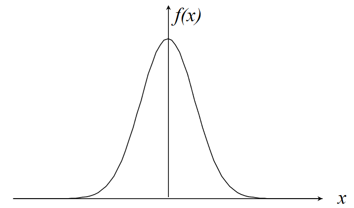
Standardised Normal Distribution
is a random variable with distribution . The standardised random variable is distributed and can be obtained with the transform: and has p.d.f.
where . Values for the standard normal distribution are tabulated in the data book.
Example
The length of bolts from a production process are distributed normally with and .
The probability the length of a bolt is between 2.6 and 2.7 cm (values obtained from table lookups):
Confidence Intervals
A confidence interval is the interval in which we would expect to find an estimate of a parameter, at a specified probability level. For example, the interval covering 95% of the population of is .
For a random variable with distribution , the standard variate . For confidence interval at 95% probability:
Using table lookups, , and:
For confidence interval at 99.9% probability:
Table lookups again, , and:
Normal Approximation to Binomial Distribution
The normal distribution gives a close approximation to the binomial distribution, provided:
- is large
- neither nor are close to zero
- and
For example, take a random process consitsting of 64 spins of a fair coin and . The probability of 40 heads is:
For a normal approximation, must use the interval around 40 (normal is continuous, binomial is discrete) :
Normal Approximation to Poisson Distribution
The normal distribution gives a close approximation to the binomial distribution, provided:
- is large
For example, say a radioactive decay emits a mean of 69 particles per seconds. A standard normal approximation to this is:
The probability of emitting particles in a second is therefore:
Equations
Below are some of the main equations that I have found useful to have on hand.
Integration and Differentiation
Cheatsheet
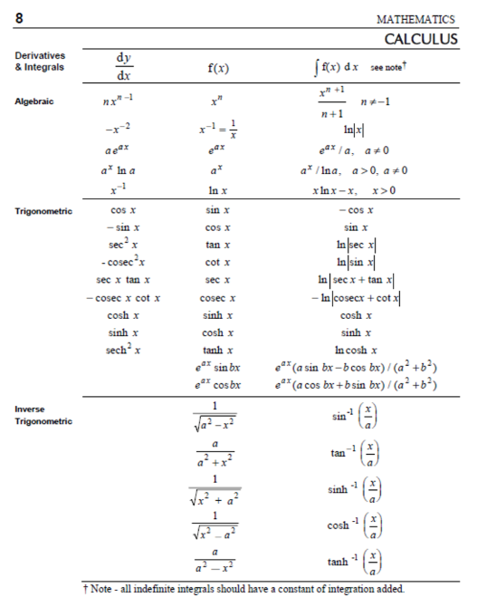
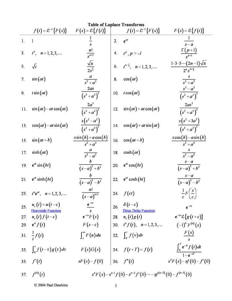
ES197
This section, similar to ES191, also aims to be fairly comprehensive as a reference. I probably won't cover much of the matlab/simulink stuff.
Translational Mechanical Systems
- Translational systems involve movement in 1 dimension
- For example, a the suspension in a car going over bumps going up and down
- System diagrams can be used to represent systems
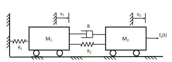
- Diagrams include:
- Masses
- Springs
- Dampers
Elements
There are element laws to model each of the three elements involved in mechanical systems. They are modelled using two key variables:
- Force in newtons ()
- Displacement in meters ()
- Also sometimes velocity in meters per second ()
When modelling systems, some assumptions are made:
- Masses are all perfectly rigid
- Springs and dampers have zero mass
- All behaviour is assumed to be linear
Mass
- Stores kinetic/potential energy
- Energy storage is reversible
- Can put energy in OR take it out
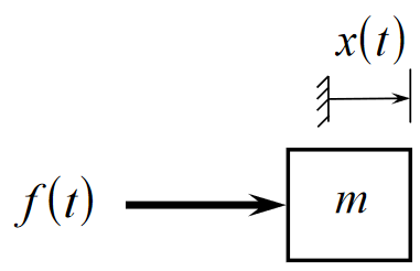
Elemental equation (Newton's second law):
Kinetic energy stored:
Spring
- Stores potential energy
- Also reversible energy store
- Can be stretched/compressed
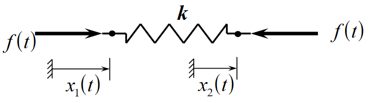
Elemental equation (Hooke's law):
The spring constant k has units . Energy Stored:
In reality, springs are not perfectly linear as per hooke's law, so approximations are made. Any mechanical element that undergoes a change in shape can be described as a stiffness element, and therefore modelled as a spring.
Damper
Dampers are used to reduce oscillation and introduce friction into a system.
- Dissapates energy as heat
- Non reversible energy transfer
- Takes energy out of the system
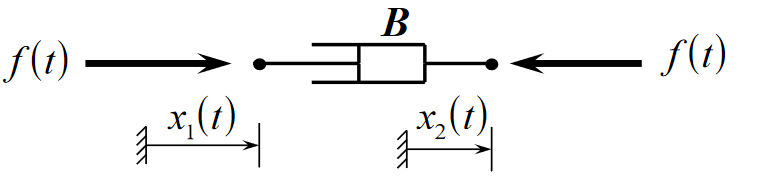
Elemental equation:
B is the damper constant and has units
Interconnection Laws
Compatibility Law
- Elemental velocities are identical at points of connection
Equilibrium Law
- Sum of external forces acting on a body equals mass x acceleration
- All forces acting on a body in equilibrium equals zero
Fictitious/D'alembert Forces
D'alembert principle is an alternative form of Newtons' second law, stating that the force on a body is equal to mass times acceleration: . is the inertial, or fictitious force. When modelling systems, the inertial force always opposes the direction of motion.
Example:
Form a differential equation describing the system shown below.
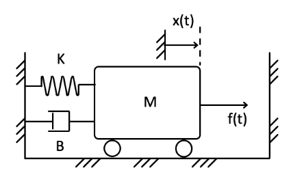
4 forces acting on the mass:
- Spring:
- Damper:
- Inertial/Fictitious force:
- The force being applied,
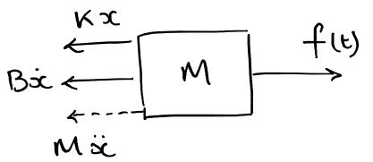
The forces all sum to zero:
Rotational Mechanical Systems
Dynamic Systems
- A system is a set of interconnected elements which transfer energy between them
- In a dynamic system, energy between elements varies with time
- Systems interact with their environments through:
- Input
- System depends on
- Do no affect environment
- Output
- System does not depend on
- Affects Environment
- Input
- Mathematical models of dynamic systems are used to describe and predict behaviour
- Models are all, always approximations
Lumped vs Distributed Systems
- In a lumped system, properties are concentrated at 1 or 2 points in an element
- For example
- Inelastic mass, force acts at centre of gravity
- Massless spring, forces act at either end
- Modelled as an ODE
- Time is only independent variable
- For example
- In a distributed system, properties vary throughout an element
- For example, non-uniform mass
- Time and position are both independent variables
- Can be broken down into multiple lumped systems
Linear vs Non-Linear Systems
- For non-linear systems, model is a non-linear differential equation
- For linear systems, equation is linear
- In a linear system, the resultant response of the system caused by two or more input signals is the sum of the responses which would have been caused by each input individually
- This is not true in non-linear systems
Discrete vs Continuous Models
- In discrete time systems, model is a difference equation
- output happens at discrete time steps
- In continuous systems, model is a differential equation
- output is a continuous function of the input
Rotational Systems
Rotational systems are modelled using two basic variables:
- Torque measured in
- A twisting force
- Analogous to force in Newtons
- Angular displacement measured in radians
- Angular velocity
- Analogous to displacement in meters
Element Laws
Moment of Inertia
- Rotational mass about an axis
- Stores kinetic energy in a reversible form
- Shown as rotating disc with inertia , units
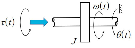
Elemental equation:
Energy Stored:
The force acts in the opposite direction to the direction the mass is spinning
Rotational Spring
- Stores potential energy by twisting
- Reversible energy store
- Produced torque proportional to the angular displacement at either end of spring
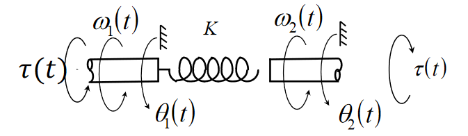
Elemental Equation:
Stored Energy:
Rotational Damper
- Dissapates energy as heat
- Non-reversible
- Energy dissapated angular velocity
Elemental Equation:
Interconnection Laws
Compatibility Law
Connected elements have the same rotational displacement and velocity
Interconnection Law
D'alembert law for rotational systems:
is considered an inertial/fictitious torque, so for a body in equilibrium, .
Example
Form an equation to model the system shown below.
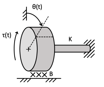
4 torques acting upon the disk:
- Stiffness element,
- Friction element,
- Input torque
- Inertial force
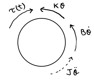
The forces sum to zero, so:
Electrical Systems
Similar to mechanical systems, models of electrical systems can be constructed. Similar deal to ES191.
Variables
- Current in amps (A)
- Voltage in volts (V) -- not v for voltage, e is used in systems
- Power in watts
Elements
Capacitors
- Store electrical energy in a reversible form
- Capacitance measured in Farads (L)
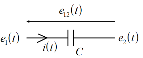
Elemental equation:
Energy stored:
Inductors
- Store magnetic energy in a reversible form
- Inductance measured in Henries (H)
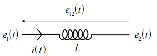
Elemental equation:
Energy Stored:
Resistors
- Dissapates energy
- Non-reversible
- Resistance measured in Ohms ()
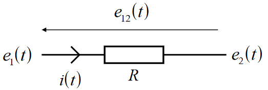
Elemental Equation (Ohm's law):
Voltage Source
- Provides an input of energy to the system.
- Input voltage
Kirchhoff's Laws
- Describe how elements interconnect and transfer energy between them
- KVL - voltages around a closed loop sum to zero
- KCL - currents about a node sum to zero
Example
Form a differential equation to model the following electrical system/circuit:
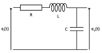
Elements:
- Resistor:
- Capacitor:
- Inductor:
KVL - the voltages round the loop sum to zero:
Using the capacitor equation, and the fact that :
Thermal Systems
- User to model heat transfer
- For example in a house
- Or in electronic components
- Determine efficiency of elements
- Determine thermal operating ranges for components
Variables
-
Rate of heat flow in watts ()
-
Temperature, in Kelvins (K)
-
Analogous to current and voltage in electrical systems
Elements
Thermal Capacitor
- Stores heat energy in a reversible way
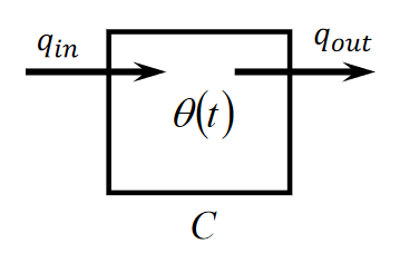
Elemental equation:
Where is the net heat flowing in, ie .
Thermal Resistor
- Dissapates heat
- Non-reversible
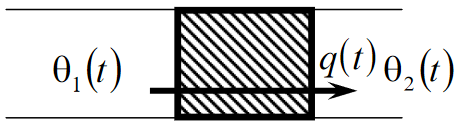
Any object that restricts heat flow when heat flows from on medium to another can be modelled as a resistor. Elemental equation:
Where is the flow of heat from the temperature on one side of the resistor to the temperature on the other.
Interconnection Laws
Compatibility Law:
- Temperatures are identical where elements touch,
Equilibrium Law:
- Elemental heat flow rates sum to zero at connection points
Examples
Develop a thermal model for someone doing winter sports. Assume:
- Ambient temperature
- Body temperature
- Thermal resistance between body and ambient (the person is wearing a coat)
- Heat generated by body
The rate of heat flow out is the difference in ambient and body temperature accross the resistor:
In the thermal capacitor, the net input heat is proportional to the rate of change of temperature:
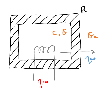
Combining the two equations gives:
Data Driven Models
- A system model can be developed from data describing the system
- Computational techniques can be used to fit data to a model
Modelling Approaches
White Box
- A white box model is a physical modelling approach, used where all the information about a system and its components is known.
- For example: "What is the voltage accross a 10 resistor?"
- The value of the resistor is known, so a mathematical model can be developed using knowledge of physics (Ohm's law in this case)
- The model is then tested against data gathered from the system
Grey Box
- A grey box model is similar to white box, except where some physical parameters are unknown
- A model is developed using known physical properties, except some parameters are left unknown
- Data is then collected from testing and used to find parameted
- For example: "What is the force required to stretch this spring by mm, when the stiffness is unknown"
- Using knowledge,
- Test spring to collect data
- Find value of that best fits the data to create a model
- Final model is then tested
- Physical modelling used to get the form of the model, testing used to find unknown parameters
- This, and white box, is mostly what's been done so far
Black box
"Here is a new battery. We know nothing about it. How does it performance respond to changes in temperature?"
- Used to build models of a system where the internal operation of it is completely unknown: a "black box"
- Data is collected from testing the system
- An appropriate mathematical model is selected to fit the data
- The model is fit to the data to test how good it is
- The model is tested on new data to see how closely it models system behaviour
Modelling in Matlab
Regression
- Regression is predicting a continuous response from a set of predictor values
- eg, predict extension of a spring given force, temperature, age
- Learn a function that maps a set of predictor variables to a set of response variables
For a linear model of some data :
- and are the predictor variables from the data set
- and are the unknowns to be estimated from the data
- Polynomial models can be used for more complex data
In Matlab
% data points
x = 0:0.1:1.0;
y = 2 * x + 3;
%introduce some noise into the data
y_noise = y + 0.1*randn(11,1)';
%see the data
figure;
plot(x,y_noise);
axis([0 1 0 5])
In matlab, the polyfit function (matlab docs) is used to fit a polynomial model of a given degree to the data.
- Inputs: x data, y data, polynomial degree
- Output: coefficients of model
P = polyfit(x,y_noise,1) % linear model
hold on;
plot(x,polyval(P,x),'r');
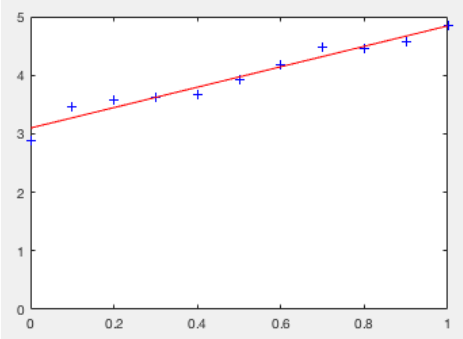
In the example shown, the model ended up as , which is close, but not exact due to noise introduced into the data.
Limitations
- Too complex of a model can lead to overfitting, where the model contains unwanted noise
- To overcome this:
- Use simpler model
- Collect more data
First Order Step Response
Modelling is about predicting the behaviour of a system. Often, need to know
- What is the output for a given input?
- Is the system stable?
- If the input changes quickly, how will the output change?
First Order Systems
First order systems are those with only one energy store, and can be modelled by a first order differential equation.
| Type | Equation |
|---|---|
| Electrical | |
| Thermal | |
| Mechanical | |
| General |
For the general form of the equation , the solution for a step input at time , with : T is the time constant of the system.
Free and Forced Response
- Free response:
- The response of a system to its stored energy when there is no input
- Zero Input
- Non-zero initial Conditions
- Homogenous differential equation
- Forced response:
- The response of a system to an input when there is no energy initially in the system
- Non-zero input
- Zero initial Conditions
- Non-homogeneous differential equation
- Total system response is a linear combination of the two
System Inputs
Different inputs can be used to determine characteristics of the system.
Step Input
- A sudden increase of a constant amplitude input
- Can see how quickly the system responds
- Is there is any delay/oscillation?
- Is it stable?
Sine Wave
- Can vary frequency and amplitude
- Shows frequency response of a system
Impulse
- A spike of infinite magnitude at an infinitely small time step
Ramp
- An input that starts increasing at a constant rate, starting at .
Step Response
- The step response of the system is the output when given a step input
- System must have zero initial conditions
- Characteristics of a response:
- Final/resting value
- Rise time
- Delay
- Overshoot
- Oscillation (frequency & damping factor)
- Stability
For a system with time constant , the response looks something like this:
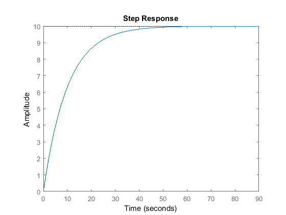
The time constant of a system determines how long the system takes to respond to step input. After 1 time constant, the system is at about (63) % of its final value.
| Time (s) | % of final value |
|---|---|
| 39.3% | |
| 63.2% | |
| 86.5% | |
| 95.0% | |
| 98.2% | |
| 99.3% |
Second Order Step Response
How 2nd order systems (those with 2 energy storing elements) respond to step inputs.
Standard form
- is the undamped frequency of the system response
- Indicates the speed of the response
- is the damping factor
- Indicates the shape of the response
Forced Response
- Forces response is the response to a non-zero input, namely
- Step
- Sinusoidal
- Initial conditions are zero, it ,
- The response is the solution to a non-homogeneous second order differential equation
Damped Response
There are 4 different cases for system response:
| Damping Factor | Response |
|---|---|
| No Damping | |
| Underdamped | |
| Critically Damped | |
| Overdamped |
The response of a system to the same input with varying damping factors is shown in the graph below, from the data book. The equations are also given in the data book.
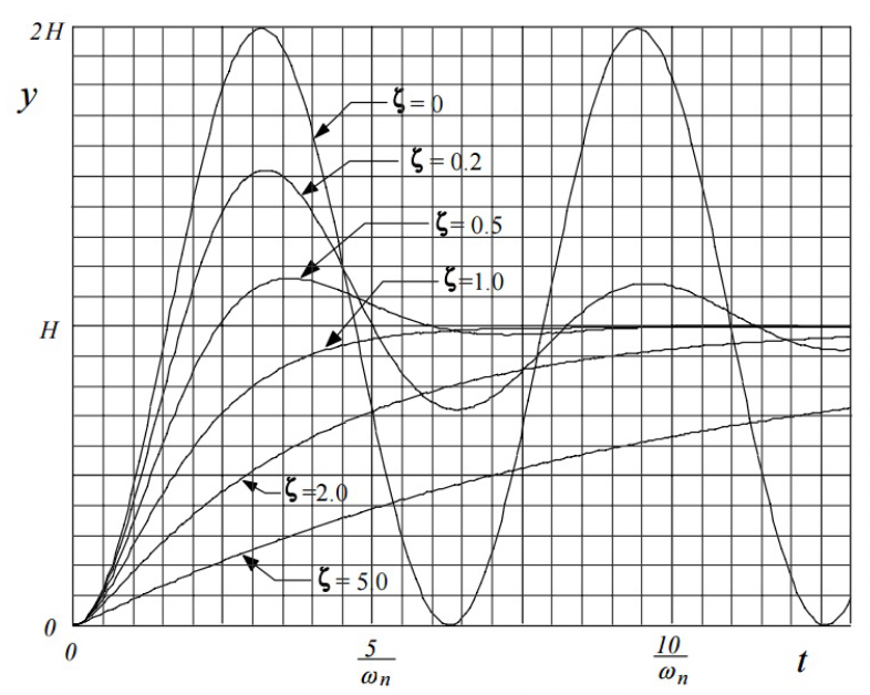
Undamped
The system is not damped at all and is just a normal sinusoidal wave.
Underdamping
The amplitude of the sinusoidal output decreases slowly over time to a final "steady state" value.
Critical Damping
This gives the fastest response, where the output rises to its final steady state value.
Overdamping
The output rises slowly to its steady state value
Transfer Functions
- A transfer function is a representation of the system which maps from input to output
- Useful for system analysis
- Carried out in the Laplace Domain
The Laplace Domain
- Problems can be easier to solve in the Laplace domain, so the equation is Laplace transformed to make it easier to work with
- Given a problem such as "what is the output given a differential equation in and the step input ?"
- Express step input in Laplace domain
- Express differential equation in Laplace domain and find transfer function
- Find output in Laplace domain
- Transfer back to time domain to get
| Function | Time domain | Laplace domain |
|---|---|---|
| Input | ||
| Output | ||
| Transfer |
The laplace domain is particularly useful in this case, as a differential equation in the time domain becomes an algebraic one in the Laplace domain.
Transfer Function Definition
The transfer function is the ratio of output to input, given zero initial conditions.
For a general first order system of the form
The transfer function in the Laplace domain can be derived as:
Step Input in the Laplace Domain
Step input has a constant value for
For a first order system, the output will therefore be:
Example
Find the transfer function for the system shown:
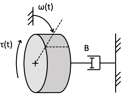
The system has input-output equation (in standard form):
Taking the Laplace transform of both sides:
Rearranging to obtain the transfer function:
Using Matlab
In matlab the tf function (Matlab docs) can be used to generate a system model using it's transfer function. For example, those code below generates a transfer function , and then plots it's response to a step input of amplitude 1.
G = tf([1],[2 3]);
step(G);
Example
For the system shown below, where , , , plot the step response and obtain the undamped natural frequency and damping factor .
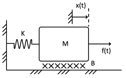
system = tf([1],[100 40 100]);
step(system, 15); % plot 15 seconds of the response
%function to obtain system parameters
[wn,z] = damp(system)
The script will output wn=1, and z = 0.2. The plotted step response will look like:
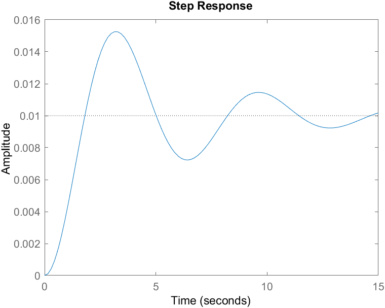
First Order Frequency Response
Frequency response is is the response of a system to a sinusoidal/oscillating input.
Response to Sinusoidal input
For a standard first order system , with a sinusoidal input :
The sinusoidal part of the equation is the steady-state that the response tends to, and the exponential part is the transient part that represents the rate of decay of the offset of the oscillation.
- The frequency of input and output is always the same
- It is the amplitude and phase shift that change
- These depend on the input frequency
- This dependence is the frequency response
Example
The example below shows an input , and its output with
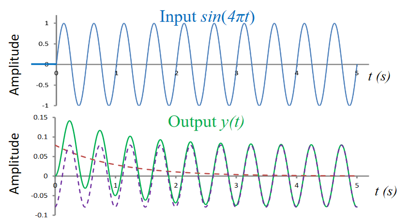
The steady state sinusoidal and transient exponential part of this response can be seen in the equation.
Matlab Example
The following code generates the following plot
system = tf(1,[1 1]);
t = 0:0.01:3; % time value vector
u = (t>=1).*sin(4 * pi * t) %input signal for t >= 1
y = lsim(sys,u,t); % simulate system with input u
figure;
subplot(2,1,1); plot(t,u); title("input");
subplot(2,1,2); plot(t,y,'r'); title("outputA");
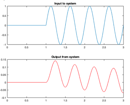
Gain and Phase
Gain is the ratio of output to input amplitude, ie how much bigger or smaller the output is compared to input.
Phase difference is how much the output signal is delayed compared to the input signal. Both are functions of input frequency .
The frequency response can be obtained by substituting for in the transfer function. This gives a complex function as shown
Magnitude gives the amplitude of the response, and the argument of the complex number gives the phase shift . The substitution is used, is because in the Laplace domain, both signals and systems are represented by functions of .
- The -plane is the complex plane on which Laplace transforms are graphed.
- Generally,
- is the Neper frequency, the rate at which the function decays
- is the radial frequency, the rate at which the function oscillates
- Periodic sinusoidal inputs are non decaying, so , giving
To find the frequency response parameters:
The graphs below show the frequency response in terms of for varying frequency :
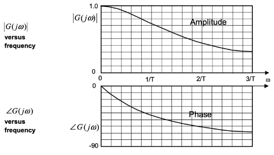
Example
Given a transfer function , what is the magnitude and phase of frequency response?
Bode Plots
Bode plots show frequency and amplitude of frequency response on a log scale. Information is not spread linearly accross the frequency range, so it makes more sense to use a logarithmic scale. An important feature of bode plots is the corner frequency: the frequency at the point where the two asymptotes of the magnitude-frequency graph. This point is where .
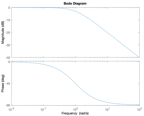
The plot above is for the function . The gain is measured in decibels for the magnitude of the response.
Second Order Frequency Response
How second order systems respond to sinusoidal/oscillating input. Similar to first order.
Gain and Phase for Second Order Systems
For a 2nd order system in standard input-output form:
The gain and phase of the frequency response are therefore:
Bode Plots, from Data Book
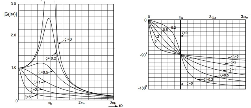
The plots show gain and phase shift for varying values of
Example
For the electrical system shown below with the values , , find:
- The undamped natural frequency
- The damping factor
- Sketch the magnitude of the frequency response
- At what frequency is this at it's maximum?
- Sketch a bode plot using matlab
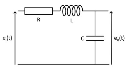
The system equation is:
Undamped natural frequency:
Damping factor:
Using the graph from the data book
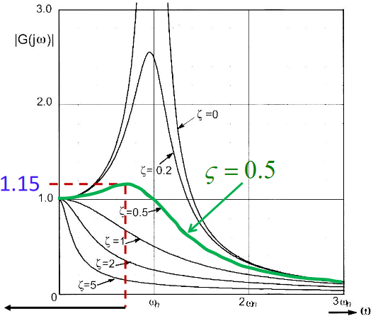
The graph peaks at approx , so:
Matlab plot:
R = 1000
C = 10e-7
L = 0.1
sys = tf([1],[L*C R*C 1]); figure; step(sys);
bode(sys);
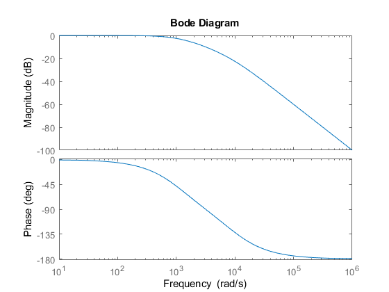
CS241
Operating Systems
Processes
- Process is a program in execution
- A process in memory has
- Text: process instructions
- Data: global variables
- Stack & Heap
- Can shrink/grow at runtime
- Process can be in several states
- New: being created
- Ready: waiting to be assigned to processor
- Waiting: waiting on something or other
- Running
- Terminated: finished execution
- Process control blocks
- Stores:
- State
- Program counter
- CPU registers
- Scheduling info
- Memory management info
- Accouting information
- CPU usage, time since start, etc
- I/O Status
- Open files and I/O devices
- Stored in kernel memory
- Used when saving processes for context switches
- Simpler the PCB, faster the context can switch
- Stores:
- Process scheduling
- Scheduler selects among available processes for who's turn is next on the CPU
- Three queues:
- Job queue for new processes (long term)
- Ready queue for ready processes (short term)
- Device queues for processes waiting for I/O access
- Short term scheduler selects next process from ready queue
- Invoked frequently and must be fast
- Long term moves from new state to ready queue
- Invoked when processes are created
- Moves processes into memory
- Not used in modern OS
- Process creation
- Child processes can be created by parent processes
- Forms a tree
- Root process is
init
- Options are specified when creating process
- Resource sharing options
- Execution options (concurrently or parent waits)
- Address space options (duplicate or child loads new)
fork()creates new process as duplicateexec()used after fork to replace address space with new program
- Child processes can be created by parent processes
- Process termination
- Processes terminate after executing last statement
- Can be terminated with
exit()syscall, returning status code wait()tells parent to wait for child to exit- If a parent exits without waiting for child, children become orphans and are adopted by
init - When a process terminates but exit code has not yet been collected it is a zombie process
- All resources released but entry in process table remains
- Once parent gets exit status it is released
- Inter-process communication
- Either shared memory or message passing
- Shared memory
- Address space of one process and other one attaches to it
- Special permission required for one process to access another's address space
mmap()syscall creates shared block of memory
- Message passing
- Send and receive syscalls provided
- One process typically act as producer and other consumer
- Message buffer exists in kernel space
- Circular queue can be used as a shared buffer
- Can have zero-capacity, or bounded/unbounded
- Can communicate directly by naming processes
- Can also communicate indirectly using mailboxes
- Mailboxes have unique IDs
- Process can only communicate if they share a mailbox
- Can do blocking sends/receives, or non-blocking
- Pipes
- A mechanism for message passing in UNIX
- Pipes in bash exist with
|, connecting input of one process to output of another - Named pipes, or fifos appear in file system and can be manipulated using file operations
- Much more powerful, persist beyond processes exiting
Threads
- What are threads
- A unit of CPU execution
- Can multi-thread processes to achieve concurrency
- Threads lighter than processes and share more with parent
- Share code, data, files
- Threads have own id, program counter, register set, stack (share heap)
- Concurrency and parallelism
- Concurrency implies more than one task making progress
- Parallelism implies that a system can perform more than one task simultaneously
- Data parallelism splits data up and performs same processing on each subset of data
- Task parallelism splits threads doing different things up
- Can have concurrency without parallelism by interleaving tasks on one core
- Amdahl's law is a rough estimate of speedup
- Speedup
- Numerator (1) is time taken before parallelising
- is time taken to run serial part
- is the time taken to run parallelisable part on cores
- Pthreads is common API for working with threads
pthread_create()creates new thread to execute a functionpthread_join()waits for thread to exit- Provides mutexes and condvars
- Can set thread IDs and work with attributes, etc
- Synchronising threads
- Sharing memory between threads requires synchronisation
- Race conditions occur when two threads try to write to a variable at the same time
- High level code broken down into atomic steps which become interleaved and cause registers and intermediate operations to become mixed up, causing undefined behaviour
- Can use mutexes for synchronisation
- User vs Kernel threads
- User level threads are implemented by user code in userspace
- No kernel involvement
- Cannot be scheduled in parallel but can run concurrently
- Kernel threads are implemented by the kernel and created by syscalls
- Scheduling is handled by kernel so can be scheduled on different CPUs
- Management has kernel overhead
- Many-to-one model maps many user level threads to a single kernel thread
- Less overhead
- User threads are all sharing kernel thread so no parallelism and one blocking causes all to block
- One-to-one gives each user thread a kernel thread
- Used in windows and linux
- More kernel threads = more overhead
- Users can cause creation of kernel threads which slows system
- Many-to-many multiplexes user threads across a set of kernel threads
- Number of kernel thread can be set and can run in parallel
- More complex than one-to-one
- User level threads are implemented by user code in userspace
- Condition variables
- Used to synchronise threads
- Threads can
wait()on condition variables - Other threads signal the variable using
signal()orbroadcast()
- Signals are used in UNIX systems to notify processes
- Synchronous signals generated internally by process
- Asynchronous signals generated external to process by other processes
- ctrl+c sends SIGINT asynchronously
- Signals are delivered to process and handled by signal handlers
- Only signal-safe functions can be called within signal handlers
- Signals can be delivered to all threads, just the main thread, or specific threads
Scheduling
- Different schedule queues contain processes in different states
- Queues contain process control blocks
- Scheduler wants to be as efficient as possible in scheduling jobs
- Maximise CPU utilisation and process throughput
- Minimise turnaround, waiting, response times
- Four events that can trigger scheduler
- Process switches from running to waiting state
- Process terminates
- Process switches from running to ready
- Process switches from waiting to ready
- First two cases are non pre-emptive, where process give up CPU
- 2nd two are pre-emptive, where scheduler takes the task off the CPU and gives it to a new task
- First-come first-serve scheduling is where processes are assigned to CPU in order of arrival
- Avg wait time varies massively on order of processes arriving
- Non pre-emptive
- Shorter jobs first improves performance
- Shortest first scheduling
- Provably optimal in minimising average wait time
- Relies on knowing how long each job will take
- Can estimate job length by exponential moving average
- is the length of the nth CPU burst
- is the predicted length of the next CPU burst
- Can be either pre-emptive or non pre-emptive
- When a new, shorter process arrives when one is already being executed, can either:
- Switch to new process
- Wait for current job to finish
- Pre-emptive can cause race conditions where processes are switched mid-write
- When a new, shorter process arrives when one is already being executed, can either:
- Priority scheduling assigns a priority to each process, and lowest priority is executed first
- Shortest job first is a special case of priority scheduling, where the priority is execution time
- Can cause starvation for processes with low priority
- Can overcome with aging, where priority is increased over time
- Round robin scheduling is where each process gets a small amount of CPU time (a quantum ), and after that time has elapsed the process is pre-empted and put back into the ready queue
- Scheduler visits process in arrival order
- No process waits more than for it's next turn
- If is large, becomes first come first served
- If is small, too many context switches
- usually 10 to 100ms
- Higher wait time than shortest job first in most cases, but better response time
Synchronisation
- Synchronisation is important to prevent race conditions
- Needed for both process and threads as they both share memory
- The part of code where processes update shared variables is the critical section
- No two processes can concurrently execute their critical section
- Entry and exit must uphold mutual exclusion
- No two processes can concurrently execute their critical section
- Ideal solution to the critical section problem must satisfy:
- Mutual exclusion
- At least one process must be able to progress into the critical section if no other process is in it
- No process should have to wait indefinitely to enter critical section
- Peterson's Algorithm is a solution to the problem
int turn;shared variable to specify who's turn it isboolean flag[2];flags store who wished to enter- Process runs if both waiting and their turn, or if only one waiting and other not in critical section
- Can fail with modern architectures reordering stuff
- Synchronisation primitives are based on the idea of locking
- Two processes cannot hold a lock simultaneously
- Locking and unlocking should be atomic operations
- Modern hardware provides atomic instructions
- Used to build sync primitives
- Test and set is one type of atomic instruction
- Update a register and return it's original value
- Can be used to implement a lock using a shared boolean variable
- Does not satisfy bounded waiting as the process can instantly reacquire the lock
- More complex implementations can satisfy criteria (allow the next waiting process to execute and only release lock if no other process waiting)
- Mutex locks are lock variables that only one process can hold at a time
- If another process tries to acquire the lock then it blocks until the lock is available
- Semaphores have integer values
- 0 means unavailable
- Positive value means available
wait()on a semaphore makes the process wait until the value is positive- Decrements by 1 if/when positive
signal()increments value by one- Both commands must be atomic
- Controls the number of processes that can concurrently access resource - more powerful than mutex
- Deadlocks may occur when both processes are waiting for an event that can only be caused by the other waiting process
- Starvation occurs when a specifics process has to wait indefinitely while others make progress
- Priority inversion is a scheduling problem when a lower-priority process holds a lock needed by a higher priority process
- Solved via priority inheritance, where the priority of the low priority task is set to highest to prevent it being pre-empted by some medium priority task.
- There are a few classic synchronisation problems that can be used to test synchronisation schemes
- The bounded buffer problem has buffers where each can old one item. Produces produces items and write to buffers while the consumers consume from buffers
- Producer should not write when all buffers full
- Consumer should not consume when all buffers empty
- Solved with three semaphores
mutex = 1; full = 0; empty = n
- Producers wait on empty when filling a buffer, and signal on full to indicate a buffer has been filled
- Consumers wait on full to indicate emptying a buffer, and wait on empty to indicate one has been emptied
- buffer access protected by mutex
- Reader/writer problem has some data shared among processes, where multiple readers are allowed but only one writer
- Readers are given preference over writers, and writers may starve
- A shared integer keeps track of the number of readers, and two mutexes are used, one read/write mutex, and another to protect the shared reader count.
- The writer must acquire the writer mutex
- Readers increase the read count while reading and decrease when done, both operations synchronised using mutex
- Read/write mutex also locked while read count is at least one reading to prevent writes while anyone is reading.
- Dining philosophers spend their lives either thinking or eating.
- They sit in a circle, with a chopstick between each pair. When they wish to eat, they pick up a chopstick from either side of them, and put them back down when done.
- Two neighbouring philosophers cannot eat at the same time
- Five mutexes, one for each chopstick
- If all five decide to eat at once and pick up the left chopstick, then deadlock occurs
- There are multiple solutions:
- Allow only philosophers for chopsticks
- Allow a philosopher to only pick up both chopsticks if both are available, which must be done atomically
- Use an asymmetric solution, where odd-numbered philosophers pick up left first, and even numbers pick up right first
- They sit in a circle, with a chopstick between each pair. When they wish to eat, they pick up a chopstick from either side of them, and put them back down when done.
- The bounded buffer problem has buffers where each can old one item. Produces produces items and write to buffers while the consumers consume from buffers
Deadlocks
- A set of processes is said to be in deadlock when each process is waiting for an event that can only be caused by another process in the event
- All waiting on each other
- Usually acquisition/release of a lock or resource
- An abstract system model for discussing deadlocks
- System has resources
- Resources can have multiple instances
- A set of processses
- To utilise a resource a process must request it, use it, then release it
- System has resources
- Conditions for deadlock:
- Mutual exclusion, only one process can use a resource
- Hold and wait, a process must hold some resources and then be waiting to acquire more
- No pre-emption, a resource can be released only voluntarily
- Circular wait, there must be a subset of processes waiting for each other in a circular manner
- The resource allocation graph is a directed graph where:
- Vertices are processes and resources
- Resource nodes show the multiple instances of each resource
- Request edge is a directed edge
- Assignment edge is a directed edge
- Cycles in graph show circular wait
- No cycles means no deadlock
- Cycles may mean deadlock, but not sufficient alone to detect deadlock
- Vertices are processes and resources
- Deadlock detection algorithms are needed to verify if a resource allocation graph contains deadlock
- Resource graph can be represented in a table showing allocated, available, and requested resources
- Flags show if each process has finished executing
- A process may execute and set it's flag if it can satisfy it's requested resources using the currently available resources, which then frees any allocated resources
- Can then try to execute other processes
- If ever a point where no progress can be made, then the processes are deadlocked
- Deadlock prevention ensures that at least one of the necessary conditions for deadlock does not hold
- Impossible to design system without mutual exclusion
- Can prevent hold-and-wait by ensuring a process atomically gets either all or none of its required resources at once, so it is either waiting on one of them or all of them
- Can introduce pre-emption into the system to make a process release all it's resources if it is ever waiting on any
- Can prevent circular wait by numbering resources, and requiring that each process requests resources in order
- Process holding resource cannot request any resources numbered less than
- All of these methods can be restrictive
- Harmless requests could be blocked
- Deadlock avoidance is less restrictive than prevention
- Determines if a request should be granted based upon if the resulting allocation leaves the system in a safe state where no deadlock can ever occur in future
- Need advanced information on resource requirements
- Each process declares the maximum number of instances of each resources it may need
- On receiving a resource request, the algorithm checks if granting the resource leaves the system in a safe state
- If it can't guarantee a safe state, the system waits until the system changes into a state where the request can be granted safely
- How do we determine if a state is safe?
- Cycles alone do not guarantee deadlock
- The banker's algorithm determines if a state is safe
- Determines if a request should be granted based upon if the resulting allocation leaves the system in a safe state where no deadlock can ever occur in future
- The banker's algorithm:
- Take a system with 5 process and three resource types, A, B and C, with 10, 5, and 7 instances respectively.
- Table shows the current and maximum usage for each process
- Available resources is (instances of resource) - (total current used by each process)
- Future needed resources is (maximum usage) - (current usage)
- At each step, a process is found who's needs can be satisfied with currently available resources
- Can then execute process and reclaim its resources
- Keep applying steps to try to reclaim all resources
- Gives a sequence that processes can be executed in
- If sequence completes all processes then it's a safe sequence and starting state is safe
- If some processes cannot be executed and there is no possible safe sequence the starting state is unsafe
- Gives a sequence that processes can be executed in
- Resource request algorithm checks if granting a request is safe
- Check that we can satisfy request
- Pretend request was executed
- Use bankers algorithm to see if resulting state would be safe
- If not, then keep request pending until state changes into a safe state where we can grant it
Memory
- Memory is a flat array of addressable bytes
- CPU fetches data and instructions from memory
- Memory protection
- Addresses accessible by a process must be unique to that process such that processes cannot write to each others address spaces
- Base and limit registers define the range of legal addresses
- OS loads these registers when a process is scheduled
- Only OS can modify
- CPU checks addresses are in legal range, OS takes action if not
- Assumes contiguous memory allocations, but other methods exist
- Address binding
- Addresses in source code are usually symbolic (variables)
- Typically bound by compilers to relocatable addresses
- Addresses in object code are all mapped relative to some base address, which is then mapped to a physical address when loading into memory
- Different address binding strategies exist, can be done at compile time, load time, or execution time
- Addresses in source code are usually symbolic (variables)
- Addresses generated by a program during its runtime are either logical or physical
- Logical/virtual are generated by the CPU to fetch or read/write, may differ from physical address
- Must be converted to physical address before being used to access memory
- Physical address is the one seen by the memory unit.
- Under compile and load time binding, logical and physical addresses are the same
- Under execution time binding, the physical addresses may change at runtime
- Logical/virtual are generated by the CPU to fetch or read/write, may differ from physical address
- The memory management unit is special hardware that translates logical to physical addresses
- MMU consits of a relocation register and a limit register under contiguous allocation
- Three main techniques for memory allocation
- Contiguous memory allocation
- Each process has one chunk of memory
- Used in older OSs
- MMU checks each logical address against limit register
- Registers can only be loaded by OS when a process is scheduled
- Memory divided into fixed partitions which are allocated to processes
- Fixed number of partitions => fixed number of processes
- OS keeps track of free chunks called holes
- Processes allocated memory based on their size
- Put into a hole large enough to accommodate it
- Different strategies for hole allocation
- First-fit, allocate first hole
- Best-fit, allocate smallest hole possible
- Must search entire address space
- Worst-fit, allocate the largest hole
- Must also search entire address space
- Produces largest leftover hold
- Can result in fragmentation of the address space
- External fragmentation, when there is enough memory space for a process but it is not contiguous
- Internal fragmentation, where a process is using more memory than it needs
- Can deal with it by compacting holes into one block
- Require processes to be relocated during execution and have significant overhead
- Can also allow non-contiguous allocation
- Segmented memory allocation
- Program divided into segments, each in its own contiguous block
- Each logic address is a two-tuple of
(segment number, offset)- Segment number mapped to base address and offset is
- MMU contains segment table
- Table indexed by segment numbers
- Each table entry has
- Segment base, which is the physical address of the segment in memory
- Segment limit, the size of the segment
- Still cannot avoid external fragmentation
- Paging is the best technique for memory management
- Avoids external fragmentation
- Divide program into blocks called pages
- Divide physical memory into blocks called frames
- Page size = frame size = 4kB
- Pages are assigned to frames
- Mapping between pages and frames is stored in a page table, one for each process
- Logical addresses have a page number and a page offset
- Still suffers from internal fragmentation
- Worst case scenario has one byte in a frame
- Average wastage is half a frame
- Smaller frames means less wastage but larger page tables
- Page table implementations are complex
- There is a page table in memory for each process
- MMU consists of registers to hold page table entries
- Loaded by OS when a process is scheduled
- Can only store a limited number of entries
- Holding a page table in memory doubles the time it takes to access an address, because you need an access to translate logical -> physical address first
- Translation Lookaside Buffer (TLB) stores frequently used page table entries in a hardware cache
- Extremely fast
- On a cache miss, the entry is brought into the TLB
- Cache miss requires an extra memory access to get page table entry on top of the usual fetch
- Different cache replacement algorithms are used (LRU is common)
- Different algorithms have different corresponding hit ratios
- Effective memory access time depends on hit ratio
- Stores page table entries of multiple process
- Each entry requires an Address Space Identifier (ASID) to uniquely identify the process requesting the TLB entry
- Cache only hits if ASID matches, which guarantees memory protection
- It can be beneficial to have smaller page tables to reduce memory overhead
- 32 bit word length and 4kB page size gives possible entries
- If each entry is a 4 byte address, this is 4MB of page table per page
- Most processes only use a very small number of the logical entries
- A valid-invalid bit is used for each page table entry to indicate if there is a physical memory frame corresponding to a page number
- Bit is set high when there is no physical frame corresponding to a a page
- Hierarchical page tables divide the page table into pages and store each page in a frame in memory
- The mapping is stored in an outer page table
- The OS does not need to store the inner page tables that aren't in use
- The flat page table requires 4MB of space, which requires 1000 frames of 4kB each
- The outer page table will have 1000 entries (one for each inner page table), which fits in a single frame.
- Addressing under multi-level paging works by separating the address into chunks
- Outer and inner page tables are 4kB, so hold 1000 4 byte addresses.
- 10 upper bits address the outer page table
- Next 10 bits address the inner page table
- Lowest 12 bits used to address the 4kB address space of each page
- This takes 3 memory accesses now, which is slow
- Less memory used but higher penalty in case of TLB miss
- Outer and inner page tables are 4kB, so hold 1000 4 byte addresses.
- Hashed page tables use the page numbers as hash keys, which are hashed to the index of the page table
- Each entry is a pointer to a linked list of page numbers with the same hash value
- Each list node is the page number, frame number, and pointer to the next node
- Each entry is a pointer to a linked list of page numbers with the same hash value
- Some architectures use inverted page tables, where each index in the table corresponds to a physical frame number
- Each entry in the table is a PID and a page number
- When a virtual address is generated, each entry is searched until the entry for the frame with the page number and PID is found
- Decreases memory needed to store each page table, but increases search time
Networks
Intro
- A network is a group of interconnected dervices that communicate by sending messages
- End hosts run applications and send/receive messages
- Generate messages and break them down into packets
- Add additional info such as IP address and port in packet header
- Send bits physically
- Access points provide access to the internet
- End hosts connect to APs
- Most use ethernet/wifi but also 4G/5G mobile networks
- Intermediate devices such as switches and routers forward and route messages
- Also known as network core
- Run routing and forwarding algorithms
- Info stored in routing tables
- Move packets to correct output link
- End hosts run applications and send/receive messages
- The store-and-forward principle states that an entire packet must arrive at a before it can re-send it
- It takes seconds to transmit a packet of length at bits per second
- The router has to receive and send, so total delay is , plus processing time
- Packets queue at the router if the rate of incoming packets is greater than the transmittion rate
- Packets either queue in buffer or may be dropped if buffer fills
- There are four main sources of packet delay:
- Transmission delay
- time to send packet
- Queueing delay
- Time waiting to be transmitted
- Processing delay
- Any processing at node
- Propagation delay
- Time to physically move bits in link cables
- Transmission delay
- Throughput is the overall rate at which bits are transferred from a source to a destination in a time window
- Can be instantaneous throughput, the rate at a specific point in time
- Or average throughput, the mean rate over a longer period of time
- Transmission links are bottlenecked by their minimum speeds
- Protocols are defined rules for communication between nodes
- Define packet format, order of messages, actions to take on send and receive
- Can be in software or hardware
- Routers run IP protocols and switches and network cards implement ethernet
- The internet uses packet switching to allow different routes to share links between nodes
- If one flow of data is not using any shared links then another flow can use it
- Circuit switching was used in old telephone networks, where links were reserved for an entire call duration and flows did not get shared
- Not ideal for internet traffic due to the bursty nature of packets
- There are 5 layers in the network stack, each using the services of the layer below it and providing services to the layer above it
- Application layer generates data
- HTTP, SMTP, DNS
- Transport layer packetises data, adds port number, sequencing and error correcting info
- TCP, UDP
- Network layer adds source and destination IP addresses and routes packets
- IP
- Link layer adds source/destination MAC addresses, passes ethernet frames to network interface hardware drivers
- Ethernet, WiFi
- Physical layer sends the bits down the wire
- Different protocol for cables, WiFi, fibre optics, etc
- Application layer generates data
Application Layer
- Processes such as web browsers, email, file sharing, communicate over networks
- Developer has to develop either both client and server so they know how to communicate
- Alternatively, processes can implement an application-layer protocol such as HTTP
- Process send/receive via sockets, which are the API between application and network
- Creating, reading, writing to sockets is done by syscalls
- Messages need to be addressed to the correct process running on the correct end host
- Host identified by IP address
- Processes identified by port number
- Application processes use transport layer services
- Transport layer is expected to deliver messages to the intended recipients
- All transport layer protocols provide basic services such as packetisation, addressing, sequencing, error correction
- Different protocols provide different services
- TCP is for reliable and ordered data transfer
- Is correction-oriented
- TCP handshake is required
- Client must contact server, establish connection with IP and Port
- Provides a
- Is correction-oriented
- UDP provides no guarantees on data transfer
- Best-effort service
- Faster as no handshake is required and headers are smaller
- Maintains no connection, data may be lost or our of order
- HTTP is how web browsers communicate with web servers
- Uses TCP port 80
- Client sends a HTTP request to request a resource
- Server response with a HTTP response with the requested resource
- Web pages consist of HTML file and references objects
- HTTPv1.0 is non-persistent and downloads each object over a separate TCP connection
- New TCP handshake for each object
- HTTPv1.1 is persistent and uses the same connection for multiple objects
- Server leaves connection open for any referenced objects, which are sent back-to-back as soon as they are encountered
- RTT is the round trip time for a request
- Needs 1 RTT to establish TCP connection, then another to request and receive first few bytes of data
- Non-persistent response time is 2RTT + file transmission time for each file
- Persistent response time only requires 2RTT once, then total data transfer
- HTTP requests and responses are in ASCII, in a human-readable format
- In request, top line is request line with request verb (GET/POST/PUT)
- In response, top line is status line with status code and phrase
- Web clients can be configured to access the web via a cache, which caches objects to reduce response time for client requests
Transport Layer
- Transport services provide logical communication between application processes running on different hosts
- Break messages into segments, add header, pass to network layer on the send side
- Reassemble segments into messages and pass up to application layer on the receive side
- UDP provides bare minimum services
- No effort to recover lost packets or re-order packets
- Connectionless
- Each segment treated individually
- No congestion control
- Sender can send as fast as they want, possibly overloading receiver or infrastructure
- Used when fast and low latency is needed
- UDP header is smaller
- Can send data as fast as wanted
- Video games, internet streaming
- It is the programmers responsibility to make UDP reliable
- TCP is connection-oriented and more reliable
- Provides flow and congestion control
- Manages packets out of order to make packets appear in order
- Enhances unreliable network layer services
- Bits often flipped due to noise and packets re-ordered
- Checksums in headers detect bit errors
- Acknowledgments (ACKs) indicated packets are correctly received
- Sender times out if ACK not received within a timeout interval
- Automatic Repeat Requests (ARQs) are sent to retransmit lost or corrupt packets
- Packets include a sequence number to detect lost or duplicated packets
- Stop and wait ARQ is a protocol for ARQs
- Sender sends a packet and waits until it receives an ACK
- If ACK arrives, send the next packet
- If ACK times out, retransmit the same packet
- Duplicate detection is possible because sequence numbers are used
- Sufficient to use 1 bit sequence number since there can be at most one outstanding packet
- Known as the alternating bit protocol
- Sufficient to use 1 bit sequence number since there can be at most one outstanding packet
- Reliable, but slow as sender has to wait for ACK to send next packet
- Suppose a 1Gbps () link with a packet length of bits
- RTT is 30ms
- Utilisation is the fraction of time the link is spent transmitting
- time spent sending, time spent waiting
- The sender should be allowed to send more packets without waiting for an ACK
- There is bits of additional data that could be sent during the RTT interval
- is the delay-bandwith product
- Indicates the length of the pipeline
- Receiving buffer can also be a bottleneck
- Typically has a finite buffer of bits
- May not be reading from buffer all the time
- Sender should not send more than bits at a time to prevent overflow
- The maximum number of bits without waiting for an ACK is
- Pipelined protocols allow multiple unacknowledged packets in the pipeline
- ACKs are sent individually or cumulatively
- Range of sequence number must be increased from alternating bits
- Go-back-n is a common protocol
- Sender maintains a window of packets that can be sent without waiting for ACK
- Depends on delay-bandwith product, receive buffer size, other factors
- Receiver maintains expected sequence number variable, keeps track of the next expected packet
- If the receiver receives the packet with the expected sequence number, then it sends ACK(), which acknowledges all packets up to , making the ACK cumulative
- If the sequence number is not the expected one, then the receiver discard the incoming packet and sends ACK(), acknowledging all up to the last correctly received packet
- Waits for packet to be correctly received before acknowledging any further packets
- The sender moves the send window forward for every ACK received
- Maintains a timer for the oldest unacknowledged packet, if an ACK times out then the packet is resent
- Sender maintains a window of packets that can be sent without waiting for ACK
- Selective repeat does not discard out of order packets as long as they fall inside a receive window
- ACKs are individual and not cumulative
- Sender selectively retransmits packets whose ACK did not arrive
- Maintains a timer for each unacknowledged packet in the send window
- Does not have to retransmit out-of-order packets
- Packets arriving out of order are buffered, but receive window not moved forward
- Window size should be less than or equal to half the max sequence number
- Avoids packets being recognised incorrectly
- Send window moved forward when ACK received
- TCP uses a combination of GBN and SR protocols
- Uses cumulative ACKs
- Only retransmits the packet causing timeout
- Each byte of data is numbered in TCP
- Sequence number of a packet is the byte number of the first byte of the segment
- TCP ACK number is the number of the next byte expected from the other side
- Cumulative ACKs are used
- TCP is duplex, so ACKs are piggybacked onto data segments. A segment can carry data and serve as an ACK
- The timout period is often relatively long, so on 3 duplicate ACKs, the sender re-transmits that segment without waiting for timeout
- Duplicate ACKs are good indicators of high packet loss
- TCP headers contain a few fields
- Sequence number is the 32 bit number of the segment indicating the number of the first byte in the packet
- Acknowledgement number is the number of the next byte expected to be transmitted
- Receive window is used for flow control
- TCP uses flow control to ensure that the data in the pipeline does not exceed the receive buffer size
- Receiver advertises free buffer spaces in the receive windows field -
rwnd - Sender limits amount of unacknowledged data to the receiver's
rwndvalue - (last byte send - last byte ACK'd)
rwnd
- Receiver advertises free buffer spaces in the receive windows field -
- TCP provides congestion control to control the rate of transmission according to the level of perceived congestion in the network
- Congestion occurs when input rate > output rate
- Results in lost packets, buffer overflows, long delays due to queuing at routers
- As a transmission link approaches maximum capacity queues build up and delay approaches infinity
- There is no benefit in increasing transmission rate beyond network capacity
- In a circular network where the transmission rate via link is and the capacity of the link is
- If , then : the links can all transmit at the same rate and there is no congestion
- If , then only a portion of the traffic can be carried by each link
- The throughput increases linearly up to a max of , then decreases exponentially towards 0 from there causing congestion collapse
- Throughput control aims to limit send rates such that congestion collapse does not occur, and flows get a fair share of network resources
- TCP detects network congestion through delays and losses
- Congestion is assumed when timeout occurs or 3 duplicate ACKs are received
- TCP is a window-based pipelined protocol, where the rate of transmission is window size
- Controlling controls the transmission rate
- Maximum size of a TCP segment is the MSS, Maximum Segment Size, which is determined by the maximum frame size specified by the link layer
- Number of segments to transmit all data is
- The sender maintains a congestion window size, denoted
cwndW = LastByteSent - LastByteAcked <= min(cwnd, rwnd)- When
rwndis large, sendercwnddetermines the transmission rate, which bps
cwndis a function of perceived network congestion- Varied using additive increases and multiplicative decreases (AIMD)
- Increase
cwndby 1MSS every RTT until loss detected - Cut
cwndin half after loss - Achieves a fair allocation rate among competing flows
- Additive increase gives a slope of 1 as throughput increases
- Multiplicative decrease decreases throughput proportionally
- if no loss, if loss
- Ideal operating point for two connections sharing bandwith is that both are sending at bps
- Increase
- Varied using additive increases and multiplicative decreases (AIMD)
- TCP starts slowly as AIMD convergence rate is slow
- Window size increased exponentially until predefined threshold hit (
ssthresh)- "slow start" phase,
cwnddoubled each RTT ssthreshremembers previous window size for which a loss occurred
- "slow start" phase,
- Initial aggressive behaviour ensure sender reaches correct speed quickly
- Window size increased exponentially until predefined threshold hit (
- Losses are detected through timeouts and 3 duplicate ACKs
- Harsher on losses than duplicate ACKs
- Timeout indicates a packet loss, so drastic action is taken
ssthresh= 0.5 * cwnd,cwnd = 1 MSS- Sender enters slow start phase again
- Losses indicated by duplicate ACKs take less drastic action -
ssthresh= 0.5 * cwnd,cwnd = 0.5 * cwnd- Window grows again linearly (additively)
Network Layer
- The main function of the network layer is to move packets from the source to destination node through intermediate nodes (routers)
- Main protocol on this layer is IP
- At the source, the IP header is added with source and destination IP addresses
- Routers check destination IP addresses to decide the next hop
- At the destination, the IP header is stripped and the packet is delivered to the transport layer
- Routers have two key functions
- Forwarding, moving packets from the input to the appropriate output
- Routing, constructing routing tables and running routing protocols
- Routing tables map destination IP ranges to their output links
- Mapping all 4 billion IP addresses would be impractical
- If the IP ranges don't divide up so nicely, longest prefix matching is used
- When looking for a table entry for a given destinaion address, use the longest address prefix that matches the destination address
- IPv4 addresses are 32bits to uniquely identify network interfaces
- IP addresses belonging to the same subnet have the same prefix, the subnet mask
- Interfaces on the same subnet are connected by a link layer switch and communicate directly
- IP addresses have their subnet mask specified as the number of bits as a prefix
- CIDR notation is xxx.xxx.xxx.xxx/xx
- A sender checks if the destination IP has the same subnet mask
- If it does then obtain the MAC address of the destination and forward the packet to the link layer switch
- If source and destination belong to different subnets, then the source forwards the packet to it's default gateway
- Gateway routers connect subnets
- If
Awant so communicate withBon a different subnet, it forwards the packets toR, the default gateway Rwill look up in it's routing table to forwardA's packets to the correct outgoing interface- When the packet reaches the interface, it will be forwarded to
Bthrough the switch inB's subnet
- Nodes have two options for acquiring IP addresses
- Network admins can manually configure the IP of each host on the network
- DHCP is an application layer protocol that dynamically assigns IP addresses from the server to clients
- Both subnet mask and default gateway must be provided for both
- Networks are allocated subnets from the ISP's address space
- Global authority ICANN is responsible for allocating IP addresses to ISPs
- Network Address Translation (NAT) is used so that each IP address on a subnet does not need a globally unique IP, as ICANN have run out of them (4 billion is not enough)
- Unique IP addresses are provided to public gateway routers
- Private IP addresses that are unique only on the subnet are allocated by the gateway router
- Devices in home or private networks need not be visible to the public internet, they can use private IP addresses to communicate with each other and communication with the internet is done via the gateway router
- Packets with private IP addresses cannot be carried by the public internet
- Private source IP addresses are converted to the public IP address of the router facing the internet
- Incoming packets for different hosts are distinguished by different ports on the router
- Address shortage is solved by IPv6 with 128-bit addresses, but it is not in wide use yet
- At each router, a routing protocol such as RIP or OSPF constructs the routing table
- Each routing protocol implements a routing algorithm
- Networks are abstracted as graphs
- is the set of routers
- is the set of links
- Each edge has a cost associated with if
- if and are not direct neighbours
- The cost of a path
- The idea is that given a source and destination , what is the least cost path from to
- Need the shortest past from each node to every other node to populate the routing table
- Two type of routing algorithm are used
- Global requires the knowledge of the complete topology at each router including costs
- Link state algorithms
- Local requires only knowledge of the network surrounding the router
- Global requires the knowledge of the complete topology at each router including costs
- Dijkstra’s algorithm is a link-state routing algorithm that computes leas cost path from one node (the source) to all other nodes
- Implemented in Open Shortest Path First (OSPF) protocol
- Each node requires the entire topology, which is obtained through broadcasting link states
- Maintains a set of visited nodes , initially only the source
- For all nodes
- If adjacent to
- D(v) = c(u, v) , store current estimates of shortest distance
- p(v) = u, store predecessor node of along with current shortest path from to
- else, , , initialise all other nodes to be infinite distance away with no known predecessor yet
- If adjacent to
- While all nodes not in , not yet visited
- Add node to
- For all adjacent to and not in
- If
- , update distance to the unvisited neighbour of if it is smaller
- If
- The Distance Vector (DV) algorithm is used in the Routing Information Protocol (RIP)
- Uses local information from neighbouring nodes to compute shortest paths
- Based on the Bellman-Ford equation
- is the length of the shortest path from to
- BF equation relates to , where (the set of neighbouts of x)
-
- If minimises the above sum, then it is the next-hop node in the shortest path
- is the current estimate of the minimum distance from to (different to actual minimum distance )
- DV algorithm tries to converge estimates to their actual values
- Each node maintains a distance vector
- Node performs the update
- Node needs toe cost of each neighbour, and the distance vector of each neighbour (obtained via message passind)
- Whenever any of these is updated, the node recomputes it's distance vector and update all it's neighbours
- Each node:
- Wait for a change in local link cost or a message from neighbour
- Recompute estimates using BF equation
- If DV to any destination has changed, notify neighbours
Selected Topics
- A network interfaces is how the computer connects to a network
- Node can have multiple interfaces
- Loopback address (localhost) is simulated interface
- Each interface has an IP address
- Each NIC has a MAC address
- Internet protocols specify the structure of internet packets
- Packet headers are added at each layer of the network stack
- Ethernet header from link layer describes source and destination MAC addresses
- Fixed length header
- IP header from network layer describes source and destination IP
- Variable length header, length stored in
IHLfield - Stores protocol of transport layer too
- Variable length header, length stored in
- TCP/UDP header from transport layer has port numbers, control bits
- Also has data offset has the header length is variable
- Has sequence number, ACK number and checksum
- Application message is after the three headers
- SYN attacks are when a malicious attacker sends a flood of TCP packets with the SYN bit set
- This causes the server to reply with SYN ACK for each packet received, creating a bunch of half open connections waiting for an ACK that never arrives
- The server is then too busy to respond to any other users
- Denial of service attack
- MAC addresses are the addresses of the physical network interface hardware
- Address Resolution Protocol (ARP) determines the MAC addresses of hardware from the IP addresses
- The router broadcasts an ARP request packet to all interfaces on the link
- The ARP reply is sent by the node with the requested address
- MAC address is saved in ARP cache for future use
- ARP allows unsolicited replies from anyone, so an attacker can send an unsolicited ARP reply pretending to be another address.
- This poisons the ARP cache with an incorrect entry, and the device will the send all messages intended for the spoofed address to the attacker
CS257
Memory Systems
Main Memory
- We have a memory hierarchy to balance the tradeoff between cost and speed
- Want to exploit temporal and spatial locality
- Moore's law is long dead and never really applied to memory
- The basic element of main memory is a memory cell capable of being written or read to
- Need to indicate read/write, data input, and also an enable line
- When organising memory cells into a larger chip, it is important to maintain a structure approach and keep the circuit as compact as possible
- For example, a 16 word x 8 bit memory chip requires 128 cells and 4-bit addresses
- A 1024 bit device as a 128x8 array requires 7 address pins and 8 data pins
- Alternatively, it is possible to organise it as a 1024x1 array, which would be really dumb as it would result in a massive decoder and inefficient space usage
- Dividing the address inputs into 2 parts, column and row address, minimise the decoder space and allows more space for memory
- Can use the same principle to build smaller ICs into larger ICs, using decoders/multiplexers to split address spaces
- Semiconductor memory is generally whats used for main store, Random Access Memory
- Two main technologies:
- Static RAM (SRAM) uses a flip-flop as a storage element for each bit
- Dynamic RAM (DRAM) uses the presence or lack of charge in a capacitor for each bit
- Charge leaks away over time so needs refreshing, but DRAM is generally cheaper if the overhead of the refresh circuitry is sufficiently amortised
- SRAM typically faster so is used for cache
- DRAM used for main memory
- The interface to main memory is always a bottleneck so we can do some fancy DRAM organisations stuff
- Synchronous DRAM exchanges data with the processor according to an external clock memory
- Clock runs at the speed of the bus to avoid waiting on memory
- Processor can perform other tasks while waiting because clock period and wait times are known
- Rambus DRAM was used by Intel for Pentium and Itanium
- Exchanges data over a 28-wire bus no more than 12cm long
- Provides address and control information
- Asynchronous and block-oriented
- Fast because requests are issued by the processor over the RDRAM bus instead of using explicit R/W and enable signals
- Bus propertties such as impedances must be known to processor
- DDR SDRAM extends SDRAM by sending data to the processor on both rising and falling edge
- Actually used
- Cache DRAM (CDRAM) combines DRAM with a small SRAM cache
- Performance very dependant upon domain and load
- Synchronous DRAM exchanges data with the processor according to an external clock memory
- ROM typically used in microprogramming or systems stuff
- ROM is mask-written read only memory
- PROM is same as above, but electrically written
- EPROM is same as above, but is erasable via UV light at the chip level
- EEPROM is erasable electrically at the byte-level
- Flash memory is a high speed semiconductor memory
- Used for persistent storage
- Limited to block-level erasure
- Uses typically 1 transistor per bit
Interleaved Memory
- A collection of multiple DRAM chips grouped to form a memory bank
- banks can service requests simultaneously, increading memory read/write rates by a factor of
- If consecutive words of memory are stored in different banks, the transfer of a block of memory is sped up
- Distributing addresses among memory units/banks is called interleaving
- Interleaving addresses among memory units is known as -way interleaving
- Most effective when the number of memory banks is equal to number of words in a cache line
Virtual Memory
- Virtual memory is a hierarchical system accross caches, main memory and swap that is managed by the OS
- Locality of reference principle: addresses generated by the CPU should be in the first level of memory as often as possible
- Use temporal, spatial, sequential locality to predict
- The working set of memory addresses usually changes slowly so should maintain it closest to CPU
- Performance measured has hit ratio (assuming a two-level memory hierarchy with data in and )
- The average access time
- When there is a miss, the block is swapped in from to then accessed
- is the time to transfer a block, so
- , the access time ratio of the two levels
- , the factor by which average access time differs from minimum, access efficiency
- Memory capacity is limited by cost considerations, so wastins space is bad
- The efficiency which space is being used can be defined as the ratio of useful stuff in memory over total memory,
- Wasted space can be empty due to fragmentation, or inactive data that is never used
- System also takes up some memory space
- Virtual memory space is usually much greater than physical
- If a memory address is referenced that is not in main memory, then there is a page fault and the OS fetches the data
- When virtual address space is much greater than physical, most page table entries are empty
- Fixed by inverted hashed page tables, where page numbers are hashed to smaller values that index a page table where each entry corresponds to physical frames
- Hash collisions handled by extra chain field in the page table which indicates where colliding entry lives
- Lookup process is:
- Hash page number
- Index the page table using hash. If the tag matches then page found
- If not then check chain field and go to that index
- If chain field is null then page fault
- Average number of probes for an inverted page table with good hashing algorithm is 1.5
- Practical to have a page frame table with twice the number of entries than frames of memory
- Segmentation allows programmer to view memory as multiple address spaces - segments
- Each segment has its own access and usage rights
- Provides a number of advantages:
- Simplifies dynamic data structures, as segments can grow/shrink
- Programs can be altered and recompiled independently without relinking and reloading
- Can be shared among processes
- Access privileges give protection
- Programs divided into segments which are logical parts of variable length
- Segments make up pages, so segment table used to get offset of address within page table
- Two levels of lookup tables, address split into 3
- Translation Lookaside Buffer (TLB) holds most recently reference table entries as a cache
- When TLB misses, there is a significant overhead in searching main memory page tables
- Average address translation time
- TLB miss ratio usually low, less than 0.01
- Page size has an impact on memory space utilisation factor
- Too large, then excessive internal fragmentation
- Too small, then page tables become large and reduces space utilisation
- is the segment size in words, so when , the last page assigned to a segment will contain on average words
- Size of the page table associated with each segment is approx words, assuming each table entry is 1 word
- Memory overhead for each segment is
- Space utilisation is therefore
- Optimum page size =
- Optimum utilisation =
- Hit ratio increases with page size up to a maximum, then begins to decrease again
- Value of yielding max hit ratios can be greater than the optimum page size for utilisation
- When a page fault occurs, the memory management software is called to swap in a page from secondary storage
- If memory is full, it is necessary to swap out a page
- Efficient page replacement algorithm required
- Doing it randomly would be fucking stupid, might evict something being used
- FIFO is simple and removes oldest page, but still might evict something being used
- Clock replacement algorithm modifies fifo, which keeps track of unused pages through a
usebit- Use bit is set if page hasn't been used since last page fault
- LRU algorithm works well but complex to implement, requires an
agecounter per entry- Usually approximated through
usebits set at intervals
- Usually approximated through
- Working set replacement algorithm keeps track of the set of pages referenced during a time interval
- Replaces the page which has not been referenced during the preceding time interval
- As time passes, a moving window captures a working set of pages
- Implementation is complex
- Thrashing occurs when there is too many processes in too little memory and OS
- Get a better page replacement algorithm
- Close some chrome tabs
- Download more RAM
Cache
- Cache contains copies of sections of main memory and relies of locality of reference
- Objective of cache is to have as high a hit ratio as possible
- Three techniques used for cache mapping
- Direct, maps each block of memory to only one possible cache line
- Associative, permits each main memory block to be loaded into any line of cache
- Cache control logic must examine each cache line for a match
- Set associative, each cache line can be in one of a set of cache lines
- In direct mapping, address is divided into three fields: tag, line and word
- Cache is accessed with the same line and word as main memory
- Tag is stored with data in the cache
- If tag matches that of the address, then that's a cache hit
- If a miss occurs, the new data and tag is fetched to cache
- Simple and inexpensive
- Fixed cache location for each block means that if two needed blocks map to the same line than cache will thrash
- Victim cache was originally proposed as a solution
- A fully associative cache of 4-16 lines sat between L1 and L2
- Fully associative cache scheme divide the CPU address into tag and word
- Cache accessed by same word
- Tag stored with data, have to examine every tag to determine if theres a cache miss
- Complex because of this
- Set associative combines the two, where a given block maps to any line in a given set
- eg, a 4-way cache has 4 lines per set and a block can map to any one of these 4
- Performance increases diminish as set size increases
- Performance can be improved with separate instruction and data caches, L1 usually split
- Principle of inclusion states that L1 should always be subset of L2, L2 subset of L3, etc
- When L3 is fetched to, data is written to L2 and L1 also
- Writing to cache can result in cache and main memory having inconsistent data
- It is necessary to be coherent if
- I/O operates on main memory
- Processors share main memory
- There are two common methods for maintaining consistency
- With write through, every write operation to cache is repeated to main memory in parallel
- Adds overhead to write to memory, but usually there are several reads between each write
- Average access time
- Assumes is time to transfer block to cache, and is the fraction of references that are writes
- Main memory write operation must complete before any further cache operations
- If size of block matches datapath width, then whole block can be transferred in one operation,
- If not, then transfers are required and
- If size of block matches datapath width, then whole block can be transferred in one operation,
- Write through often enhanced by buffers for writes to main memory, freeing cache for subsequent accesses
- In some systems, cache is not fetched to when a miss occurs on a write operation, meaning data is written to main memory but not cache
- Reduces average access time as read misses incur less overhead
- With write back, a write operation to main memory is performed only at block replacement time
- Increases efficiency if variables are changed a number of times
- Simple write back refers to always writing back a block when a swap is required, even if data is unaltered
- Average access time becomes
- x2 because you write the block back then fetch a new one
- Tagged write back only writes back a block if the contents have altered
- 1-bit tag stored with each block, and is set when block altered
- Tags examined at replacement time
- Access time
- is the probability a block has been altered
- Write buffers can also be implemented
- With write through, every write operation to cache is repeated to main memory in parallel
- It is necessary to be coherent if
- Most modern processors have at least two cache levels
- Normal memory hierarchy principles apply, though on an L2 miss data is written to L1 and L2
- With two levels, average access time becomes
- A replacement policy is required for evicting cache lines in associative and set-associative mappings
- Most effective policy is LRU, implemented totally in hardware
- Two possible implementations, counter and reference matrix
- A counter associated with each line is incremented at regular intervals and reset when the line is referenced
- Reset every time line is accessed
- On a miss when the cache is full, the line with a counter set at the maximum value is replaced and counter reset, all other counters set to 0
- A counter associated with each line is incremented at regular intervals and reset when the line is referenced
- Reference matrix is based on a matrix of status bits
- If lines to consider, then the upper triangular matrix of a matrix is formed without the diagonal, with
- When the th line is referenced, all bits in the th row are set to one and th column is zeroed
- The least recently used one is one that has all 0s in its row and all 1s in its column
- There are three types of cache miss:
- Compulsory, where an access will always miss because it is the first access to the block
- Capacity, where a miss occurs because a cache is not large enough to contain all the blocks needed
- Conflict, misses occurring as a result of blocks not being fully associative
- Sometimes a fourth category, coherency, is used to describe misses occurring due to cache flushes in multiprocessor systems
- Performance measures based solely on hit rate don't factor in the actual cost of a cache miss, which is the real performance issue
- Average memory access time = hit time + (miss rate x miss penalty)
- Measuring access time can be a more indicative measure
- There are a number of measures that can be taken to optimise cache performance
- Have larger block sizes to exploit spatial locality
- Likely to reduce number of compulsory misses
- Will increase cache miss penalty
- Have a larger cache
- Longer hit times and increased power consumption and more expensive
- Higher levels of associativity
- Reduces number of conflict misses
- Can cause longer hit times and increased power consumption
- Multilevel Caches
- Idea is to reduce miss penalty
- L1 cache keeps pace with CPU clock, further caches serve to reduce the number of main memory accesses
- Can redefine average accesstime for multilevel caches: L1 hit time + (L1 miss rate x (L2 hit time + (L2 miss rate x L2 miss penalty)))
- Prioritising read misses over writes
- Write buffers can hold updated value for a location needed on a read miss
- If no conflicts, then sending the read before the write will reduce the miss penalty
- Optimisation easily implemented in write buffer
- Most modern processor do this as cost is low
- Avoid address translation during cache indexing
- Caches must cope with the translation of virtual addresses to physical
- Using the page offset to index cache means the TLB can be omitted
- Imposes restrictions in structure and size of cache
- Controlling L1 cache size and complexity
- Fast clock cycles encourage small and simple L1 caches
- Lower levels of associativity can reduce hit times as they are less complex
- Way prediction
- Reduce conflict misses
- Keep extra bits in cache to preduct the block within the next set of the next cache access
- Requires block predictor bits in each block
- Determine which block to try on the next cache access
- If prediction correct then latency is equal to direct mapped, otherwise at least an extra clock cycle required
- Prediction accuracy commonly 90%+ for 2-way cache
- Pipelined access
- Effective latency of an L1 cache hit can be multiple cycles
- Pipelining allows to increase clock speeds and bandwith
- Can incur slower hit times
- Non-blocking cache
- Processors in many systems do not need to stall on a data cache miss
- Instruction fetch could be performed while data fetched from main memory following a miss
- Allows to issue more than one cache request at at time
- Cache can continue to supply hits immediately following a miss
- Performance hard to measure and model
- Out-of-order processors can hide impact of L1 misses that hit L2
- Processors in many systems do not need to stall on a data cache miss
- Multi-bank caches
- Increase cache bandwith by having multiple banks that support simultaneous access
- Ideal if cache accesses spread themselves accross banks
- Sequential interleaving spreads block addresses sequentially accross banks
- Critical word first
- A processor often only needs one word of a block at a time
- Request the missing word first and send it to the processor, then fill the remainder of the block
- Most beneficial for large caches with large blocks
- Merging write buffer
- Write buffers are used by write-through and write-back caches
- If write buffer is empty then data and full address are written to buffer
- If write buffer contains other modified blocks then address can be checked to see if new data and buff entry match, and the data is combined with the buffer entry
- Known as write merging
- Reduces miss penalty
- Hardware prefetching
- Put the data in cache before it's requested
- Instruction prefetches usually done in hardware
- Processor fetches two blocks on a miss, the missed block and then prefetches the next one
- Prefetched block put in instruction stream buffer
- Compiler driven prefetching
- Reduces miss rate and penalty
- Compiler inserts prefetching instructions based on what it can deduce about a program
- Compiler can make other optimisations such as loop interchange and blocking
- Have larger block sizes to exploit spatial locality
Processor Architecture
CPU Organisation & Control
- Processor continuously runs fetch-decode-execute cycle
- Each instruction cycle take several CPU clock cycles
- Requires interaction of lots of CPU components
- ALU, CU, PC, IR, MAR, MDR
- Machine instructions may specify
- Op code
- Source operand reference
- Result operand reference
- Next instruction reference
- Some CPU registers are user-visible, such as data and address registers
- Control and status registers are used by CU and privileged OS processes only
- Executing an instruction may involve one or more operands, each requiring to be fetched
- Can account for this in instruction cycle model known as indirect cycle
- Instruction pipelining allows to use wasted time, as new inputs can be accepted before previously accepted instructions and been output
- Control unit is responsbible for generating control signals to drive cycle
- Observe opcode input and choose right control signal - decode
- Assert control signals - execute
- Two approaches to CU design:
- Hardwired
- Uses a sequencer and a digital logic circuit that produces outputs
- Fast but limited by complexity and inflexibility
- Microprogrammed
- Uses a microprogram memory
- Has it's own fetch-execute cycle - mini computer in the CPU
- Microaddress, MicroPC, MicroIR, microinstructions
- Easy to design, implement, flexible, can be reprogrammed
- Slower than hardwired
- Hardwired
- Instruction sequencing is important to be designed to utilise as many memory cycles as possible, possibly by overlapping fetches
- Proper sequence must be followed in sequencing control signals, to avoid conflicts
- MAR <- PC must precede MBR <- Memory
- Proper sequence must be followed in sequencing control signals, to avoid conflicts
- Micro-ops are enabled by control signals to transfer data between registers/busses and perform arithmetic or logical operations
- Each step in the operation of a larger machine instruction is encoded into a micro-instruction
- Micro-instructions make up the micro-program
- Micro-program word length is based on 3 factors:
- The max number of simultaneous micro-ops supported
- How control info is represented/encoded
- How the next micro-instruction address is specified
- Horizontal/direct control has very wide word length with few micro-instructions per machine instruction
- Outputs buffered/gated with timing signals
- Fewer instructions == faster
- Vertical control uses narrower instructions with control signals encoded into bits
- Limited ability to express parallelism
- Requires external decoder to identify what control lines are being asserted
Performance
- M J Flynn in 1966 defined a simple means of classifying machines, SISD is one such classification
- Uses fetch-decode-execute
- Fetch sub-cycle is fairly constant-ish speed
- Execute sub-cycle may vary in speed greatly
- A simple measure of performance is MIPS, millions of instructions per second
- Not actually that useful as it measures how fast a processor can do nothing
- Parallel performance is very difficult to measure due to system architecture and degree of parallelism varying
- Instruction bandwith measures the instruction execution rate, similar to MIPS
- Data bandwith measured in FLOPS measures the throughput
- It is nigh-on impossible to get full theoretical throughput in any system, especially parallel
- Speedup is a useful measure that factors in the degree of parallelism
- (Execution time on sequential machine, ) / (Execution time on parallel machine, )
- A closeley related measure is efficiency,
- Both measures depend on parallelism of algorithm
- An algorithm may be characterised by it's degree of parallelism , which is the degree of parallelism that exists at time
- Assume all computations are of two types, vector operations of length and scalar operations where
- is the total proportion of scalar ops, so is the measure of parallelism in the program
- is the throughput of vector ops in MFLOPS and is the scalar throughput
- Average throughput
Pipelining
- The problem with an instruction/execute pipeline is contention over memory access
- Overcome with interleaved memory
- Two possible methods of controlling the transfer of information between pipeline stages
- Asynchronously using handshake signals
- Most flexible, max speed determined by slowest stage
- Synchronously, where there are latches between each stage all synced to a clock
- Asynchronously using handshake signals
- Example 5-stage I/E pipeline: fetch instruction, decode instruction, fetch operands, execute instruction, store results
- Pipelining assumes the only interaction between stages is the passage of information, but there are 3 major things that can cause hazards and stall the pipeline
- Structural hazards, resource conflicts where two stages wish to use the same resource, ie a memory port
- Interleave memory or prefetch data into cache
- Control hazards occur when there is a change in order of execution of instructions, eg when there is a branch or jump
- Cause the pipeline to stall and have to refill it
- Strategies exist to reduce pipeline failures due to conditional branches
- Instruction pre-fetch buffers, which fetches both branches
- Complex and rarely used
- Pipeline freeze strategy, which freezes the pipeline when it receives a branch instruction
- Simple, but poor performance
- Static prediction leverages known facts about branches to guess which one is taken
- 60% of all branches are taken, so may be better to predict this
- However to not take wastest less pipeline cycles so average performance may be better
- Dynamic prediction predicts on the fly for each instruction
- Based on branch instruction characteristics, target address characteristics, and branch history
- Instruction pre-fetch buffers, which fetches both branches
- Data hazards, where an instruction depends on the result of a previous instruction that has not yet completed
- Structural hazards, resource conflicts where two stages wish to use the same resource, ie a memory port
- Pipeline clock period is determined by the slowest stage, usually execution
- Pipeline execution unit separately or have multiple execution units
- Sometimes useful to add feedback between stages (recursion), where the output of one stage becomes the input to a previous one
- Used in accumulation
- Alternative designs are always possible, which come with their own performance tradeoffs
- Space-time diagrams show pipeline usage
- Efficiency = (busy area)/(total area)
- Speedup
- More generally,
- is number of stages, is instructions executed
- As , $S(n) \to \n$
- Efficiency = (busy area)/(total area)
- Complex pipelines with feedback and differently clocked stages can be difficult to design and optimise
- Reservation tables are space-time diagrams that show where data can be admitted to the pipeline
Xs in adjacent columns of the same row show that stages operate for more than one clock period- More than one
Xs in a row not next to each other show feedback - Pipelines may not accept initiations at the start of every clock period, or collisions may occur
- Potential collisions shown by the distance in time slots between
Xs in each row
- Potential collisions shown by the distance in time slots between
- Collision vector is derived from the distance between
Xs-
- , always
- if a collision would occur with an initiation cycles after a previous initiation
- The initial collision vector is the state of the pipeline after the first initiation
- Distances between all pairs of
Xs in each row, if distance is then set bit
- Distances between all pairs of
-
- Need a control mechanism to determine if new initiations can happen without a collision occurring
- Latency is the number of clock periods between initiations
- Average latency is the number of clock periods between initiations over some repeating cycle
- Minimum average latency is the smallest possible considering all possible sequences of initiations
- The goal for optimum design
- A pipeline changes state as a result of initiations, so represent activity as a state diagram
- A diagram of all pipeline states and changes starting with the initial collision vector
- Shifting the collision vector to the right gives the next state
- If shifted vector has , cannot initiate
- If , then can do new initiation, new vector is bitwise OR of shifted vector and initial vector
- State diagram can be reduced to show only changes where initiations are taken
- Numbers on edges indicate number of clock periods to reach the next tate shown
- Can identify cycles in graph
- Always taking initiations when , to give minimum latency is the greedy strategy
- Will not always give minimum average latency but is close
- Often more than one greedy cycle
- Average latency for a greedy cycle is less than or equal to the number of 1s in the initial collision vector
- Gives an upper bound on latency
- Minimum average latency is greater than or equal to the max number of
Xs in any reservation table row- Gives a lower bound on latency
- Max
Xs in row min avg latency greedy cycles avg latency number of 1s in the initial collision vector
- A given pipeline may not give the required latency, so insert delays into the pipeline to expand the number of time slots and reduce collisions
- Can identify where to place delays to give a latency of cycles: -
- Start with the first
X, enter anXin a revised table and mark as forbidden every cycles, to indicate the positions are reserved for initiations - Repeat for all
Xs untilXfalls on a forbidden mark, then delay theXby one or more - Mark all delayed positions and delay all subsequent
Xs by the same amount
- Start with the first
- Delays can be added using a latch to delay by a cycle
- Reservation tables are space-time diagrams that show where data can be admitted to the pipeline
Honestly just check the slides and examples for this one it makes zero sense lol
Superscalar Processors
- A single, linear instruction pipeline provides at very best a steady-state Clocks per Instruction (CPI) of 1
- Fetching/decoding more than one instruction per clock cycle can reduce the CPI below 1
- An easy way to do this is to add duplicate the pipeline
- For example:
- Two fetch/decode stages
- Execution staging window register
- Multiple execution pipelines for different instructions
- Non-uniform superscalar has pipeline is not duplicated
- Number of replications before window is the degree of the superscalar processor
- Some pipeline stages need less than half a clock cycle, so double internal clock speed can get two tasks done per half a clock cycle
- Known as superpipelining
- A pipeline takes clock cycles to execute instructions
- A superscalar pipeline takes to do the same
- An example pipeline has 4 stages, fetch, decode, execute, write-back
- Each stage is duplicated
- , the number of replications
- , the number of stages
- If instructions are aligned, the number of clocks required if
- If instructions are unaligned, then
- Each stage is duplicated
- The CPI of a superscalar processor is
- For large values of , the speedup is limited by delays set by and pipeline length
- As increases, speedup increases linearly too until the point where instruction level parallelism limits further increases
- For many problems, ILP gives parallelism in the range 2-4x
- No reason to have a huge number of duplicated pipelines, as most programs have a limited degree of inherent parallelism
- Can be maximised by compiler and hardware techniques
- Limited by dependencies
- The program to be executed is a linear stream of instructions
- Instruction fetch stage includes branch prediction to form a dynamic stream which may include dependencies
- Processor dispatches instructions to be executed according to their dependencies
- Instructions are conceptually put back into sequential order and results recorded - known as committing or retiring the instruction
- Needed as instructions are executed out of order
- Instruction may also be executed speculatively and not need to be retired
Instruction Level Parallelism
- Common instructions can be initiated simultaneously and executed independently
- Superscalar processors rely on this ability to execute instructions in separate pipelines, possibly out-of-order
- Multiple functional units for multiple tasks
- ILP refers to the degree to which instructions can be executed in parallel
- Common techniques to exploit it include instruction pipelining and superscalar execution, but also:
- Out-of-order execution
- Register renaming
- Values conflict for use of the registers, processor has to stall to resolve conflicts
- Can treat the problem as a resource conflict, and dynamically rename registers in hardware to reduce dependencies
- Use different registers to the ones that the instructions say
- Branch prediction
- Prefetch both sides of the branch, reduces delay
- Can be static or dynamic
- Speculative execution aims to do the work before it is known if results will be needed
- Relies on resource abundance to provide performance improvements
- Fiver factors fundamentally constrain ILP:
- True data dependency
- An instruction cannot execute because it requires data that will be produced by a preceding instruction
- Usually causes pipeline delays
- Procedural dependency
- Inherent to the sequential nature of execution
- Instructions following a branch have a dependency on the result of the branch
- Variable length instructions can prevent simultaneous fetching
- Resource conflicts
- Two or more instructions require a system resource at the same time
- Memories, caches, functional units, etc
- True data dependency
- A program may not always have enough inherent ILP to take advantage of the machine parallelism
- Limited machine parallelism will always inhibit performance
- Processor must be able to identify ILP
- Instruction issue refers to the process of initiating execution in the processors functional units
- Instruction has been issued once it finishes decoding and hits first execute stage
- The instruction issue policy can have a large performance impact
- Three types of instruction order are significant:
- Fetch order
- Execute order
- Order in which instructions update the contents of memory
- Issue policy can fuck with these orders to whatever extent it pleases provided the results are correct
- Three general categories for instruction issue policies:
- In-order issue with in-order completion
- Do the same as what would be done by a sequential processor
- Issuing stalls when there is a conflict on a functional unit or takes more than one cycle
- Do the same as what would be done by a sequential processor
- In-order issue with out-of-order completion
- A number of instructions may be being executed at any time
- Limited by machine parallelism in functional unites
- Still stalled by resource conflicts and dependencies
- Introduces output dependencies
- Out-of-order issue with out-of-order completion
- In-order issue will only decode up to a dependency or conflict
- Further decouple decode and execute stages
- A buffer - the instruction window - holds instructions after decode
- Processor can continually fetch/decode as long as window not full and execution is separate
- Increases instructions that are available to execution unit
- In-order issue with in-order completion
Parallelism
Parallel Organisation
- Flynn's Taxonomy:
- SISD
- Standard uniprocessor stuff
- SIMD
- Vector/Array Processors
- Single machine instruction executes on a number of processing elements in lockstep
- MISD
- Not really used
- MIMD
- Distributed memory systems (cluster-based)
- Communicate via message passing, very scalable
- Shared memory systems
- Communicate via memory and are easy to program but memory contention can happen
- Symmetric multiprocessors
- NUMA
- Distributed memory systems (cluster-based)
- SISD
- Vector computers employ lots of arithmetic pipelines for SIMD processing
- Instructions operate on vectors of numbers (one or two dimensional)
- One operation specified for all elements of the vector
- 2 main types of architecture:
- memory-to-memory
- register-to-register (specific vector registers)
- Chaining often used - chain pipelines together for operations such as FMA
- Connect inputs/outputs via crossbar switches
- SIMD array computers had good performance for specific applications, but they're old and no-one makes them anymore
- Special set of instructions broadcast to processing elements for execution
- Array computer are dead but MMX, SSE, AVX are big in x86
- ARM has NEON coprocessor, a 10-stage SIMD pipeline
- Interconnection structure are important in allowing data or memory to be shared
- In distributed memory systems, communication is in software via ethernet or infiniband
- More efficient interconnects are needed to share memory
- A shared bus allows processor and memory to share a communication network
- Need to resolve bus contention issues
- Poor reliability
- Only good for small systems
- A cross-bar switch matrix uses a matrix of interconnects
- Functional units require minimal logic
- Switch is complex, large and costly
- Potentially high bandwith, but still struggles with contention
- Static links between each processor enable dedicated communication
- More links -> better communication rate
- Different patterns have different performance properties
- Chosen architecture of links usually is a tradeoff between cost and performance
- Hypercube is a good balance
- Number of connections and links per node are a good indication of cost
- Maximum inter-node distance is an indicator of worst-case communication delay
- Can have a dedicated link for each pair but that's expensive and rarely necessary
- A shared bus allows processor and memory to share a communication network
- Multistage switching networks can be either cross-bar or cell-based
- Requirement is to connector each processor to any other processor
- Known as the full access property
- Another useful property is that connections are non-blocking
- CLOS networks (multi-stage cross-bar switches) showed that a network with 3 or more stages can be non-blocking
- A CLOS network with 2x2 cross-bar elements is known as a Benes Network, classified as cell-based
- Most cell-based networks are highly blocking but require few switches
- Requirement is to connector each processor to any other processor
Cache Coherence
- Shared memory MIMD systems are easy to program, and can overcome memory contention via cache
- Copies of the same data may now be in different places
- Cache coherence must be maintained
- A write-through policy is not sufficient as that only updates main memory
- It is necessary to update other caches too
- Possible solutions include:
- Shared caches
- Poor performance for more than a few processors
- Non-cacheable items
- Can only write to main memory, causes problems
- Broadcast write
- Every cache write request is broadcast to all other caches
- Copies either updated or invalidated, preferably the latter as it is faster
- Increases memory transactions and wastes bus bandwidth
- Snoop bus
- Suitable for single-bus architectures
- Cache write-through is used
- A bus watcher (cache controller) is used and snoops on the system bus
- Detects memory write operations, and invalidates local cached copies if main memory updated
- Directory methods
- A directory is a list of entries identifying cached copies
- Used when a processor writes to a cached location to invalidate or update other copies
- Various methods exist
- Suitably for shared memory systems with multistage or hierarchical interconnects where broadcast systems are hard to implement
- Full directory has a directory in main memory
- A set of pointers per cache and a dirty bit is used with each shared data item
- Bit set high if cache has a copy
- Each word/block/line in cache has two state bits:
- Valid bit, set if cache data is valid
- Private bit, set if processor is allowed to write to the block
- Limited directories only stored pointer for the number of caches that have the data
- Saves memory storing pointers for caches that don't have data
- Only pointers required, but each pointer must uniquely identify one of the caches
- pointers required for each pointer instead of 1 bit
- Requires bits instead of bits
- Scales much better as entries grow less than linearly
- Chained directories also attempt to reduce the size of the directory
- Use a linked list to hold directory items
- Shared memory directory entry points to one copy in a cache, from there a pointer points to next copy, so on..
- copies may be maintained
- Whenever a new copy called for, list broken and pointers altered
- A directory is a list of entries identifying cached copies
- Shared caches
- MESI is the good protocol
- Snoop bus arrangement used with a write-back policy
- Two status bits per cache line tag so it can be in one of four states
- Modified: entry valid, main memory invalid, no copies exist
- Exclusive: no other cache holds line, memory up to date
- Shared: multiple caches hold line, memory is up to date
- Invalid: cache entry is garbage
- When machine booted, all entries are invalid
- First time memory is read, block referenced is fetched by CPU 1 and marked exclusive
- Subsequent reads by same processor use cache
- CPU 2 fetches same block
- CPU 1 sees by snooping it is no longer alone and announces it has a copy
- Both copies marked shared
- CPU 2 wants to write to the block
- Puts invalidate signal on bus
- Cached copy goes into modified state
- If block was exclusive, no need to signal on bus
- CPU 3 wants to read block from memory
- CPU 2 has the modified block, so tells 3 to wait while it writes it back
- CPU 1 wants to write a word in the block (cache)
- Assuming fetch on write, block must be read before writing
- CPU 1 generates a Read With Intend To Modify (RWITM) sequence
- CPU 2 has a modified copy so interrupts the sequence and write to memory, invaliding it's own copy
- CPU 1 reads block from memory, updates it and marks it modified
- All read hits do not alter block state
- All read misses cause a change to shared state
- Intel and AMD took different approaches to extending MESI
- Intel uses MESIF
- Forward state is a specialised shared state
- Serving multiple caches in shared state is inefficient, so only the cache with the special forward state responds to requests
- Allows cache-to-cache speeds
- AMD uses MOESI
- Owned state is when a cache has exclusive write rights, but other caches may read from it
- Changes to line are broadcast to other caches
- Avoids writing dirty line back to main memory
- Modified line provided from the owning cache
- Owned state is when a cache has exclusive write rights, but other caches may read from it
- Intel uses MESIF
Data Level Parallelism
- The utilisation of SIMD depends on applications having a degree of data-level parallelism
- Matrix oriented computation
- Image and sound processing
- Sequential thinking but parallel processing makes it easy to reason about
- Vector-specific architecures make SIMD easy but practicality is limited
- Reduced fetch/decode bandwith as fewer instructions
- Programmers view is:
- Transfer data elements to register files
- Essentially compiler-managed buffers for data
- Fixed length buffer to store a single vector
- Eg, each register holds 64 words
- Needs enough ports to service all functional units
- Ports connect to functional units over crossbar switch
- Operate on register files
- Functional units heavily pipleined
- Integrated control units detect structural or data hazards
- Also provide scalar units to compute addresses
- Can be chained with vector units
- Place results back in memory
- Transfer data elements to register files
- Loads and stores are pipleined
- Program pays memory latency cost just once, instead of once per data element
- Three contributing performance factors are:
- Length of vector ops
- Structural hazards
- Data dependencies
- Performance can be considered in terms of vector length or initiation rate
- Modern vector computers employ parallel pipelines known as lanes
- Superscalar architecture
- Convoys are sets of vector instructions that can execute together
- Performance of code sections can be estimated by counting number of convoys
- Need to ensure no structural hazards exist
- A chime refers to the unit of time to execute a single convoy
- A vector sequence of convoys executes in chimes
- Approximation ignores processor specific overhead and allows to readon about inherent data-level parallelism
- Chaining can be used to acheive performance, as it allows operations to be initiated as soon as individual elements of the vector source are available
- Earliest implementations work in a similar way to forwarding in scalar pipelines
- Flexible chaining allows a vector instruction to chain to almost any other active vector instruction
- Have to take care not to introduce hazards
- Supported by modern architectures
- A number of techniques can be applied to optimise vector architectures
- Can have multiple lanes, a single vector instruction can be split up to execute accross the lanes
- Doubling lanes but halving clock rate does not change speed
- Increases size and energy consumption
- Vector length registers vary the size of the vector operations
- Value cannot be greater than the max vector length, the physical register size
- Strip mining is a technique that generates code such that each vector operation is done for a size less than or equal to the max vector length
- Vector mask registers allow for conditional execution of each element operation, when usually conditionals would be needed that hinder performance
- Memory banking spreads memory accesses across multiple memory banks to improve the start up time for a vector load
- Can have multiple lanes, a single vector instruction can be split up to execute accross the lanes
- MMX/SSE/AVX provide SIMD in x86
- Many media applications operate on a narrower range of data types than 32-bit processors are designed for
- 8-bit colour components
- 16-bit audio samples
- A 256-bit adder can operate on 32 8-bit values at once
- MMX was introduced by intel in 1996
- Used 64-bit FP registers to provide 8 and 16-bit operations
- SSE was introduced as the successor, adding 128-but wide registers
- AVX introduced in 2010 adds 256 bit registers with a focus on double precision FP
- AVX-512 introduced doubles register size again
- Focus of SIMD extensions is to accelerate carefully implemented code
- Low cost to use
- Require little extra state compared to vector architectures
- No virtual memory problems
- Many media applications operate on a narrower range of data types than 32-bit processors are designed for
- GPUs are powerful vector units that are similar to vector architectures
- Hardware designed for graphics but usually supplemented to improve the performance of a wider range of applications
- Heterogeneous execution model
- CPU is host, GPU is device
- NVIDIA have CUDA for programming, OpenCL is vendor-independent
- GPUs provide high levels of every form of parallelism, but it is hard to achieve performance as must also manage
- Scheduling of computation
- Transfer of data to GPU memory
- CUDA threads are the lowest form of parallelism, one associated with each data element
- Can group thousands of threads to yield other forms of parallelism
- Threads organised into blocks, multithreaded SIMD processor executed a whole thread block
- Blocks organised into grids, executed independently and in any order
- GPU hardware handles thread management
Multicore Systems
- Can consider the performance of a processor in terms of the rate at which it executes instructions
- MIPS = freq * IPC
- Leads to an focus on increasing clock frequency and processor efficiency
- We've kinda hit a ceiling with this
- Alternative approach is multithreading
- Divide instruction stream into smaller streams to execute threads in parallel
- Various designs and implementations
- Threads may or may not be the same as software threads in multiprogrammed OS
- A process is an instance of a running program
- Processes own resources in their virtual address space
- Processes are scheduled by the OS
- Process switch is an operation that switches the processor form one process to another
- A thread is a unit of work within a process
- Thread switch switches processor control from one to another within the same process
- Far less costly than processes & process switches
- Implicit multithreading is the concurrent execution of multiple threads from a single sequential program
- Statically defined by compiler or dynamically in hardware
- Rarely done as it hard
- Most processors have adopted explicit multithreading, which concurrently execute instructions form different threads by either:
- Uses separate program counter for each thread
- Instruction fetching happens per thread
- Each thread treated and optimised separately
- Multiple approaches:
- Interleaved, where processor deals with more than one at a time, switching at each clock cycle
- Thread skipped when blocking
- Blocking or coarse grained, where threads execute successively until an event occurs that may cause a delay
- Delay prompts a switch to another thread
- SMT, where instructions are issues from multiple threads to the execution units of a superscalar processor
- Performance comes from superscalar capability combined with multiple thread contexts
- Chip multiprocessing replicates entire processor on same chip
- Multicore
- Interleaved, where processor deals with more than one at a time, switching at each clock cycle
- Interleaved and blocked do not provied true concurrency, whereas SMT and multicore are actual simultaneous execution
- Multicore systems combine multiple cores on a single die
- Each core has its own components (ALU, registers, PC) and caches
- Pollack's rule: performance increase is roughly proportional to square root of increase in complexity
- If we double the logic, will deliver 40% perf boost
- Multicore has potential for near-linear improvement but is hard to acheive
- Main variables are number of cores, and levels and amount of shared cache
- Can have dedicated L1/L2
- Can share L2 or have dedicated L2 and share L3
- Shared L2 cache has advantages over reliance on dedicated cache
- Constructive interference can reduce miss rates
- Data shared is not replicated in shared cache
- Amount of shared cache for each core is dynamic
- Interprocessor communication can happen through cache
- Confines cache coherence problem to L1 cache
- Clusters
- A group of interconnected whole computers working together as a unified computing resource, that creates the illusion of a single machine
- Alternative to multiprocessing for high performance and availability
- Attractive for servers
- Absolute and incremental scalability, high reliability, superior price/performance ratio
- High-speed interconnects needed
- With uniform memory access, all processors have access to all the memory in uniform time
- NUMA, Non Uniform Memory Access, gives different access times to different processors for different regions of memory
- All processors can still access all memory, just slower
- Cache Coherent NUMA (CC-NUMA) extends NUMA with cache coherence between the processors
- Used because SMP approaches don't scale, and allows for transparent-system wide memory
- Could motivate clusters, but clusters are hard to program effectively
- NUMA, Non Uniform Memory Access, gives different access times to different processors for different regions of memory
Thread Level Parallelism
- Synchronisation primitives exist in hardware that allow high-level synchronisation constructs to be built
- Establish building blocks to build actual constructs used by programmers
- Most important hardware provision is the atomic instruction
- Uninterruptible and capable of incurring value change
- May actually be an atomic instruction sequence
- In high-contention sequence, synchronisation can become a performance bottleneck
- Atomic exchange is a primitive that swaps a value in a register for a value in memory
- Can be used to build locks for synchronisation
- Assume a value of 0 indicates the lock is free, 1 indicates it is unavailable
- Simplest possible situation where two processors both wish to perform an atomic exchange
- One processor will enter the exchange first
- This processor will ensure that a value of 1 is returned to any other processor that next attempts an exchange
- The two simultaneous exchange operations will be ordered by write serialisation mechanisms
- Can be used to build locks for synchronisation
- Older microprocessors feature a test-and-set atomic instruction in hardware
- Allowed to define a test against which a value can be tested
- Value modified if defined test succeeded
- Some current gen microprocessors have fetch-and-increment atomic
- Return the value at a pointer and increment it
- Atomic instructions usually consist of some read and write
- Requiring an uninterruptible read-write fucks with a good number of things
- Cache coherence
- Instruction pipelining
- Cache performance
- Possible to have a pair of atomic instructions where the second instruction returns a value that indicates if the pair executed atomically
- Pair includes a special load known as load linked, followed by a special write, store conditional
- If they memory location specified by load linked is accessed prior to the store conditional then the store fails
- Also fails if there is a context switch
- Can implement atomic exchange using this
- If the store conditional returns a value indicating failure, then a branch jumps back and retries
- Can also implement fetch-and-increment
- Maintain a record of the address specified by linked load in a link register
- If an interrupt occurs or cache block containing address is invalidated, register is cleared
- Conditional store checks register for address matching to determine success
- To avoid deadlock, only register to register operations are permitted between linked-store instructions
- Pair includes a special load known as load linked, followed by a special write, store conditional
- Spin locks are locks that processors repeatedly attempt to required
- Effective when low latency required and lock held for short periods
- Processors with cache coherence provide a convenient mechanism for spin locks
- Testing the status of a lock requires local cache access rather than main memory access
- Temporal locality decreases lock acquisition times
- Linked-store can avoid needless bus access when multiple processors attempt to acquire a lock
- Cache coherence ensures multiple processors have a consistent view of memory, so allows communication through shared memory
- Shared memory communications means we only need consider the rules enforced on reads and writes of different processors
- Don't need to sync everything
- Shared memory communications means we only need consider the rules enforced on reads and writes of different processors
- Different models of memory consistency exist
- Simplest is sequential consistency
- Requires the results of execution be the same if memory accesses of processors were kept in order and interleaved
- Ensured all processors delay memory accesses until all cache invalidations are complete
- Simple but slow
- Synchronised consistency orders all accesses to shared data using synchronisation operations
- A data reference is ordered by a synchronisation operation if, in every possible execution, a write by one processor and an access by another are separated by a pair of synchronisation operations
- Whenever a variable might be updated without ordering by synchronisation is a data rate
- There are relaxed consistency models that allow reads and writes to complete out-of-order but use synchronisation to enforce ordering
- Three general models
- A -> B denotes that A must complete before B
- Total store ordering relaxes W -> R
- Retrains ordering among writes
- Partial order store model relaxes W -> W
- Impractical for most programs
- Relaxing R -> R and R -> W happens in a variety of models, including weak ordering and release consistency
- Simplest is sequential consistency
High Performance Systems
- Symmetric Multiprocessors (SMP) is an organisation of two or more processors sharing memory
- Processors connected by bus
- Uniform memory access
- All processors are the same and share I/O
- System controlled by integrated OS
- Performant for parallel problems
- All processors are the same so if one processor goes down another is still available
- Can scale incrementally
- Most PCs use a time-shared bus but can also use multi-port memory in more complex organisations
- Clusters are an alternative to SMP
- A cluster computer is defined as a group of interconnected computers (nodes) working together as a unified resources
- High performance and availability
- Attractive for server applications
- Absolute and incremental scalability
- Superior price/performance
- High speed message links required to coordinate activity
- Machines in a cluster may or may not share disks
- Cluster middleware provides a unified system image to the user
- Responsible for load balancing, fault tolerance, etc
- Desireable to have:
- A single entry and control point/workstation
- Single file hierarchy
- Single virtual networking
- Single memory space
- Single job-management system
- Single UI
- Single I/O space
- Single Process space
- Check pointing, to save the process state and intermediate results
- Process migration, to enable load balancing
- Both clusters and SMP provide multiple processors for high-demand applications
- SMP easier to manage and configure, take up less space and power
- Bus architecture limits processors to around 16~64
- Clusters dominate high-performance server market
- Scalable to 1000s of nodes
- SMP easier to manage and configure, take up less space and power
- Uniform memory access used in SMP organisations
- Memory access time varies in NUMA systems
- NUMA with no cache coherence is more or less a cluster system
- CC-NUMA is NUMA with cache coherence
- Objective is to maintain a transparent system memory while permitting multiple nodes
- Nodes each have own SMP organisations and internal busses/interconnects
- Each processor sees a single addressable memory
- Cache coherence usually done via a directory method
- Can deliver effective performance at higher levels of parallelism than SMP
- Bus traffic on any individual node is limited by bus capacity
- If many memory accesses are to remote performance degrades
- Software changes required to go form SMP to CC-NUMA systems
I/O
I/O Mechanisms
- Programmed I/O is a mapping between I/O-related instructions that the processor fetches from memory and commands that the processor issues to I/O modules
- Instruction forms depend on addressing policies for external devices
- Devices given a unique address
- When a processor, main memory and I/O share a bus, two addressing modes are possible
- Memory-mapped
- Same addres bus used for both memory and I/O
- Memory on I/O device mapped into the single address space
- Simple, and can use general-purpose memory instructions
- Portions of address space must be reserved
- Isolated
- Bus may have input and output command lines, as well as usual read/write
- Command lines specify if address is a memory location or I/O device
- Leaves full range of memory address space for processor
- Requires extra hardware
- Memory-mapped
- Instruction forms depend on addressing policies for external devices
- Most I/O devices are much slower than CPU, so need some way to synchronise
- Busy-wait polling is when CPU constantly polls I/O device for status
- Can interleave polling with other tasks
- Polling is simple but wastes CPU time and power
- When interleaved can lead to delayed response
- Interrupt-driven I/O is when devices send interrupts to CPU
- IRQs (interrupt requests) and NMIs (non-maskable interrupts)
- Interrupt forces CPU to jump to interrupt service routine
- Fast response, and does not waste CPU time/power
- Complex, and data transfer still controlled by CPU
- DMA avoids CPU bottleneck by speeding up transfer of data to memory
- Used where large amounts of data needed at high speed
- Control of system busses surrendered to DMA controller
- DMAC can use cycle stealing or force processor to suspend operation in burst mode
- DMA can be more than 10x faster than CPU-driven I/O
- Involves addition of dedicated hardware on the system bus
- Can have single Bus with a detached DMA, where all modules share the bus
- Can connect I/O devices directly to DMA, which reduces bus cycles by integrating I/O and DMA functions
- Can have separate I/O bus, DMA connected to system and I/O bus, devices connected to I/O bus
- Thunderbolt is a general purpose I/O channel developed by Apple and Intel
- Combines data, audio, video, power into single high speed connection (up to 10Gbps)
- Based on thunderbolt controller, high speed crossbar switch]
- Infiniband is an I/O spec aimed at high-end servers
- Intended to replace PCI in servers
- Provides remote storage, networking, connection
- Scalable and can add nodes as required
- PCIe is a serial interconnect between two devices
- Expansion bus standard
- Based on a number of signal lanes
- Packet based with a high bandwith
RAID
- RAID: Redundant Array of Independent Disks
- As performance increased there was a need for larger and faster secondary storage, and one solution is to use disk arrays
- Two general ways to utilise a disk array
- Data striping transparently distributes data over multiple disks to make the appear as a single large disks
- Improves I/O performance by allowing multiple requests to be serviced in parallel
- Multiple independent requests can be serviced in parallel by separate disks
- Single, multi-block requests can be serviced by disks acting in coordination
- More disks = more performance
- Improves I/O performance by allowing multiple requests to be serviced in parallel
- Redundancy duplicates data accross disks
- Allows continuous operation without data loss in case of a disk failure in an array
- Data striping transparently distributes data over multiple disks to make the appear as a single large disks
- RAID 0 - non-redundant striping
- Lowest cost as there is no redundancy
- Data is striped accross all disks
- Best write performance as no need to duplicate data
- Any 1 disk failure will result in data loss
- Used where performance is more important than reliability
- RAID 1 - mirrored
- 2 copies of all info is kept, on separate disks
- Uses twice as many disks as a non-redundant array, hence is expensive
- On read, data can be retrieved from either disk, hence gives good read performance
- If a disk fails, another copy is used
- Data can also be striped as well as mirrored, which is RAID 10
- RAID 2 - redundancy through Hamming codes
- Very small stripes are used, often single byte or word
- Employs fewer disks than mirroring by using Hamming codes, error correction codes that can correct single-but errors and detect double-bit errors
- Number of redundant disks is proportional to the log of the total number of data disks in the system
- On a single write, all data and parity disks must be accessed
- Read access not slowed as controller can detect and correct single-bit errors
- Overkill and not really used, only effective when lots of disk errors
- RAID 3 - bit-interleaved parity
- Parallel access, with data in small strips
- Bit parity is computer for the set of bits in the same position on all data disks
- If drive fails, parity accessed and data reconstructed from remaining devices
- Only one redundant disk required
- Can acheive high data rates
- Simple to implement, but only one I/O request can be executed at a time
- RAID 4 - block-interleaved parity
- Data striping used, with relatively large strips
- Bit-by-but parity calculated accross corresponding strips on each data disk, parity bits stored in the corresponding strip on parity disk
- Involves a write penalty for small I/O requests
- Parity computed by noting differences between old and new data
- Management software mut read old data and parity, then update new data and parity
- For large writes that touch all blocks on all disks, parity computed by XORing the data for each new disk
- Parity disk can become bottleneck
- RAID 5 - block-interleaved distributed parity
- Eliminates parity disk bottleneck by distributing parity accross all disks
- One of the best small read, large read, and large write performances
- Small read requests are still inefficient compared to mirroring due to need to perform read-modify-write operations to update parity
- Best parity distribution is left-symmetric
- When traversing striping units sequentially, you access each disk once before accessing any disk twice, which reduces disk conflicts when servicing a large request
- Commonly used in file servers, most versatile RAID level
- RAID 6 - dual redundancy
- Multiple disk failures require a stronger code than parity
- When disk fails, requires
- One scheme, called P + Q redundancy, uses Reed-Soloman codes to protect against up to two disk failures using a bare minimum of two redundant disks
- Three disks need to fail for data loss
- Significant write penalty, but good for mission-critical applications
- SSDs use NAND flash.
- Becoming more popular as cost drops and performance increases
- High performance I/O
- More durable than HDDs
- Longer lifespan, lower power consumption, quieter, cooler
- Lower access times and latency
- Still have some issues
- Performance tends to slow over the device's lifetime
- Flash becomes unusable after a certain number of writes
- Techniques exist for prolonging life, such as front-ending drive with cache and being used in RAID arrays
- Storage area networks are for sharing copies of data between many users on a network so anyone can access
- Must protect against:
- Drive failures - use RAID
- Power failures - have redundant power supplies (UPS)
- Storage controller failures - have dual active controllers
- System unit failures - controllers connect to multiple hosts
- Interface failures - have redundant links
- Site failures - keep backups offsite
- Flash copies produce an instantaneous copy while an application is running, eg for online backups
- Use a copy-on-write algorithm
- Remote copies are maintained at secondary sites for disaster recovery
- Can use synchronous copy, where data is copied before each command executed on host, keeping secondary copy always in sync
- Asynchronous copy is done after host executes command, which means data lags but is much more scalable and does not impact host performance
- Must protect against:
Request Level Parallelism
- Request level parallelism is an emphasis on independence of user requests for computational service
- Emphasis is on use of commodity hardware to provide parallelism at scale and capacity
- Applicable when provisioning resources at large scale
- Internet services
- Corporate infrastructure
- The Cloud
- Exploited in data centres and warehouse-scale computer systems
- Internet services are sustained by such systems
- Cloud computing founded on this premise
- Presents system design challenges
- Designing for scale and reliability
- Implementation and operation at scale
- Cost/performance balance
- Power consumption
- Environmental responsibility
- Common measure of data centre efficiency is power utilisation effectiveness
- PUE = (total facility power usage) / (IT equipment power usage)
- Must be at least 1
- Dependability is key - services typically are designed to run indefinitely
- Typical to pursue 99.99% uptime, less than 1hour down per year
- Can be realised through redundancy in temporal and spatial domains
- Usually achieved through replication of affordable hardware
- Network I/O is key, servers and warehouse systems must provide consistent network interface
- Must be able to support interactive and varying/unpredictable work loads
- Support must be provided for batch processing (likely highly data-parallel)
- Magnitude of parallelism must be considered to ensure that parallelism provided by hardware is justified
- Can support both data and request level parallelism
- Operational cost must be considered
- High performance servers often designed with best performance in mind
- Warehouses must be designed with longevity and efficiency in mind
- Exploiting economies of scale allows cloud providers to provide software and infrastructure as services
- Infrastructure as a service is the most basic cloud service model
- Cloud provider rents out machine and other resources
- Platform as a service makes a computing platform available to users
- Used by clients whose focus is software
- Underlying resources adapt to demand
- Software as a service provides access to application software in the cloud
- Uses "dumb" clients will all the power in the cloud
- Load balancing done in software
- Office 365 is prominent example
- Network as a service refers to cloud providers allowing infrastructure to be used as a network/transport layer
- Batch provessing workloads for warehouse-scale systems typically involve things like video transcode or search engine indexing
- MapReduce is a prominent example of how warehouse systems can necessitate alternative programming models
- Maps a function over each item of the input
- Exploits data-level parallelism
- Then collects outputs (reduces) using another function as an aggregation
- Generalisation of SIMD followed by a reduction
- MapReduce is a prominent example of how warehouse systems can necessitate alternative programming models
- Servers often fitted with local storage, and rely on ethernet-based exchange of data
- Potential latency penalties when crossing the local rack switch
- Alternative is network attached storage
- Can employ high-speed interconnect
Embedded Systems & Security
Embedded Systems
- Embedded software is software integrated with physical processes. The technical problem is managing time and concurrency in computational systems.
- Embedded processing is in everything, and will be in more things as computing becomes more ubiquitous
- Application areas include:
- Automotive
- ABS brakes
- ESP - electronic stability control
- Airbags
- Automatic gearboxes
- Smart keys
- Avionics
- Flight control
- Anti-collision systems
- Flap control
- Entertainment systems
- Consumer electronics
- TVs
- Smart Home
- Automotive
- Dependability is key
- Reliability is the probability of a system working correctly, provided it was working at
- Maintainability is the probability of a system working correctly time units after an error occured
- Availability is the probability of a system working at time
- Safety - no harm must be caused
- Security - data and communication must be confidential and authenticated
- Embedded systems bust be efficient:
- Code-size efficient (especially for SoCs)
- Runtime efficient
- Weight and size efficient (small)
- Cost and energy efficient
- Power is the most important constraint in embedded systems
- General purpose processors are CPUs like we're used to
- Application specific have all the same components but are more optimised with custom hardware
- Single-purpose processors have very limited resources and are constrained to run a single program
- Different types of hardware:
- ASICs - Application Specific Integrated Circuits
- Custom designed circuits on chips
- Necessary if ultimate speed or efficiency is the goal
- Can- only be produced in volume
- Masks to produce are hugely expensive
- Suffers from lack of flexibility, long design times and high costs
- Power consumption scales with voltage quadratically
- Can do dynamic power management
- Varying clock speed can save energy
- FPGAs - Field Programmable Gate Arrays
- hahaha
- DSPs - Digital Signal Processors
- MPUs - Microprocessor Units
- ASICs - Application Specific Integrated Circuits
- Minimising power consumption is important for
- Design of power supply
- Design of voltage regulators
- Dimensioning of interconnect
- Cooling - high cost and limited space
- Energy availability often restricted (battery powered)
- Lower temperatures lead to longer lifetimes
- Efficiency also a concern in memory
- Speed, must have predictable timing
- Energy efficiency
- Size
- Cost
- Energy usage and access time increases with size
- Scratch pad memory is a small separate memory mapped intro address space
- Selection done through a simple address decoder
- Used as it is far more energy efficient than a cache
Security
- Hardware typically has ports, which can be a security risk
- USB killer is a thumb drive than charges and then discharges capacitors over the data pins
- DMA provides access to memory over the system bus
- High speed expansion puts often connected to DMA
- System may be vulnerable if ports connect directly to physical address space
- Mitigated by signing drivers to verify the operation of a device
- Use IOMMU to implement virtual addressing for I/O devices
- Modify kernel to disable DMA
- Intel has a history of security concerns
- 1995 paper warned against a timing channel relating to CPU cache and the TLB
- 2012 - Apple XNU kernel adopts Address Space Layout Randomisation (KASLR)
- Linux adopted in 2014
- Primary goal to mitigate address leaks
- 2016 conference demonstrated "Using Undocumented CPU Behaviour to See into Kernel Mode and Break KASLR"
- Demonstrated techniques for locating kernel modules
- Defeated the point in KASLR
- KASLR was found to have lots of vulnerabilities, but has been updated and replaced with Kernel Page Table Isolation (KPTI)
- Work was done looking at side effects of instructions, leaking info form hardware
- Measure memory access timings
- Attacker primes cache
- Victim evicts cache
- Attacker probes data to see if it has been accessed
- Measure memory access timings
- Lots of CVEs in 2017 related to speculative execution
- Meltdown is a CVE related to rogue data cache load
- Melts security boundaries normally enforced by hardware
- Speculative out-of-order execution may execute code that is never intended to be run
- Separate side-channel attack called flush and reload can highlight what was brought into cache by speculative execution
- 3 steps:
- Attacker-chosen memory location is loaded into register
- Transient instruction accesses cache line based on register contents
- Attacker uses flush and reload to determine accessed cache line and hence the secret stored at memory location
- Accesses memory-mapped pages
- Mitigation prevents probes from revealing anything useful
- Performance impact can be very high in some workloads
- Every intel processor from 1995-2018 vulnerable
- Some ARM and IMB PowerPC too
- AMD thought to be immune, by variant discovered in 2021 that exploits branch predictor
CS261
Requirements & Software Methodologies
- Formal guidelines on how software should be engineered
- Software process model is a sequence of activities that leads to the production of a software product
- Specification - what software should do
- Design and implementation - how should be organised and implemented
- Validation and testing - does it do what it should
- Software evolution - changing software over time
- Plan driven
- All activities planned in advance
- Progress measured against plan
- Fixed, detailed spec before development commences
- Agile
- Incremental planning
- More adaptable to change
Plan-Based Methodologies
- Waterfall model has a strict linear ordering of processes
- Each stage must be completed before moving on
- If anything changes in the plan, go back to the start again
- Stages:
- Requirements analysis
- System's services, constraints, goals are established and defined
- System design
- Identification of software components and their relationships
- Implementation and unit testing
- Software programmed in unit, each unit tested against specification
- Integration and system testing
- Software components integrated and tested together as a complete system
- Operation and maintenance
- System installed, any errors that appear are fixed
- System services enhanced as new requirements added
- Requirements analysis
- Works if requirements are fixed an understood
- Fewer team constraints
- Each component can be tested against spec
- Easy to churn team because everything well-documented
- Customers can wait a long time for results
- Difficult to accommodate change
- Difficult to respond to changing requirements
- Can be a problem if project is long running
- Longer time = more likelihood of things changing
- Plan driven too rigid - introduce flexibility with incremental development
- Develop in staged with customer feedback incorporated between iterations
- Specification - development - validation is iterative
- New functionality can be added in each iteration
- Each stage planned in full and validated against plan
- Cost of accommodating change is reduced
- Software available to use quicker so feedback can be gathered easily
- Customers can see development in progress
- Easier to include user acceptance testing
- Difficult to estimate cost of development
- Difficult to maintain consistency
- As progress continues, becomes harder to include new features or make changes
- Not cost effective to document each version
- Increased cost of repeated deployment
- Re-writing software from scratch is expensive
- Rely instead on off the shelf components (libraries, frameworks)
- Include component analysis in development flow, identify library/framework
- Requirements may have to accommodate available components
Agile Methodologies
- Agile development is a principle that defines a set of methodologies
- Interleaves specification, design and implementation
- System developed as a series of versions
- Feedback provided at each stage
- Process driven approaches have become too cumbersome as businesses need to be able to evolve more rapidly
- Increased focus on code over design
- Principles include
- Customer involvement
- Incremental delivery
- People, not process
- Embrace change
- Maintain simplicity
- Focuses on development over documentation - can make it hard to pick up a system later on
- Works well as long as original team continues the evolution - problems can arise if team changes
- Possible to use techniques from both plan-based and agile, depending on what is applicable
- Extreme programming is an agile methodology involving incremental delivery with fast iteration
- Build several times a day
- Deliver to customers often
- Automate tests to verify builds
- Strong customer involvement
- Incremental planning with requirements on story cards, stories selected based on priority
- Small releases with initially minimal functionality, then building with more
- Simple design, only enough to meet current requirements
- Write tests before the software - test driven
- Developers expected to continually refactor code
- Pair programming provides support
- Collective code ownership allows for anyone to work on anything
- Continuous Integration integrates components as soon as they are ready
- Working at a sustainable pace is important for developers
- Having customer on-site is useful to incorporate frequent feedback
- Scrum is a general agile method that focuses on managing iterative development
- 3 primary stages:
- Outline planning phase to establish general goals
- Sprint cycles, each cycle developing an increment of the system
- Project closure, wrap up project, document, deliver
- Uses quick development cycles of typically 2-4 weeks
- Daily team meetings to discuss current work
- Each sprint completes item on backlog
- Features selected with customer
- Scrum master interface between team and customer
- End of each sprint, work reviewed and presented
- 3 primary stages:
Requirements Analysis
- Requirements are descriptions of what the system should and should not do, the service it provides, and the constraints on its operation
- Enable developers to make software that wil correctly fulfil customers needs
- Provides a basis for tests, validation and verification
- Enable (semi-)cost accurate specification
- Important to distinguish what is built from how it is built
- Requirements act as a bridge between customers and developers
- First stage in any process is software specification - requirements engineering
- Requires that we define the services required from the system
- Identify constraints on operation and development
- Produce a requirements document
- End user facing and system developer facing - possibly two documents
- Feasibility study determines that task is feasible and cost effective
- Requirements elicitation and analysis derives the system requirements
- Look at existing docs
- Talk to customer
- Discuss features
- Possibly prototype
- Requirements specification translates information gathered in elicitation into formal documents
- Requirements validation ensures requirements are achievable and valid
- Need to ensure customer signs off requirements
- Notion of C- and D-requirements for customer and development facing
- Technical requirements vs idiot speak
- C-requirements describe operation and constraints from users's point of view
- D-facing give detailed description of system functions, acting as basis for contract with developer
- Good requirements are
- Prioritised: features have an implementation priority
- Consistent: requirements do not conflict with each other
- Modifiable: able to revise set of requirements when necessary and maintain history of changes
- Traceable: able to link each requirement to source, which could be higher-level requirement, use case, or customer statement
- Correct: accurately describes functionality to be delivered
- Feasible: must be possible to implement each requirement within the known capabilities and limitations of environment
- Necessary: should document something that customers actually need, or is required for conformance to external standard or interface
- Unambiguous: someone reading requirement should interpret it only one way
- Verifiable: can tests or other approaches be used to verify if requirement has been implemented properly
- MoSCoW requirements group requirements into 4 groups:
- Must have
- Should have
- Could have
- Won't have
- Requirements document will be read by:
- Customers
- Managers
- Engineers
- Testers
- Maintainers
- Sections include:
- Preface - history and purpose of document
- Intro - justify and outline system
- Glossary
- User requirements design - describe services provided for users
- System architecture - high-level overview of system
- Requirements spec - describe functional and non-functional requirements
- System models - show relationships between system components
- System evolution - anticipated changes due to changing future needs
- Functional requirements describe what system should do, state system services and how it should behave in different scenarios
- Non-functional requirements are constraints on services or functions offered by system, describe qualities of the system such as availability, performance, etc
- Requirements engineering processes is not a linear sequence, processes often interleaved and iterated upon
- Requirements discovery
- Gather info from stakeholders
- Domain research
- Consider use cases
- Classification and organisation - group similar requirements and organise into categories
- Prioritisation and negotiation - assign priorities and sort conflicts between requirements from different stakeholders
- Specification - write the document and give to stakeholders, then iterate
- Requirements discovery
- Requirements validation is key once document has been written
- Validity - will system support customer's needs?
- Consistency - are there any conflicts?
- Realism - can system be produced with available resources and technology?
- Verifiability - can system be shown/proved to satisfy requirements?
- Review by both customers and engineers
- Prototyping and test-case generation
- Requirements must be managed to see if they should be accepted
- Problem analysis - is new requirement valid and unambiguous?
- Change analysis - what are the effects on the rest of the system?
- Change implementation - do the change
- Must take into account legal, social, ethical, professional issues
- Copyright
- Patents
- Developers given fair recognition of work
- Software not produced to do anything illegal or evil
- Work completed in best interest of customer
System Modelling
- UML was developed in the 90s as a general purpose modelling language, providing a formal scheme for describing system models.
- Static/structural view of system (objects and their attributes)
- Dynamic/behavioural view - dynamic behaviour of system (collaboration betwen objects and changing state)
- Different perspectives for system modelling include:
- External - the context of the system
- Interaction
- Between system and it's environment
- Between components of system
- Structural
- Organisation of system
- Structure of data being processed
- Behavioural - dynamic behaviour of the system
Structural UML
- Creating a static view of a system requires identifying entities, which can be done in one of four ways
- Grammatical approach based on natural language of the system
- Identify key items from the description of the problem
- Identification of tangible things in the application domain
- Behavioural approach to identify objects
- Scenario-based, where objects, attributes and methods in each scenario are identified
- Grammatical approach based on natural language of the system
- Class diagram shows system classes and their relationships
- Show structure of design and organisation of components
- UML formal notation move requirements closer to a mathematical description
- Forces us to think about the language used in D-requirements
- Class name is shown in diagram
- Attributes shown with types
- Methods shown with return and argument types
- Use the line with the crows foot for showing one-to-many or many-to-many
- Use ranges to indicate how many objects there are
- Writing correct class diagrams:
- Class name should be at the top
- Abstract classes go in italic
- Interfaces are represented <<interface>>
- Attributes represent internal datatypes and are optional
- Methods that make up public interface should be included
- Don't show inherited
- Don't show getters/setters
- Symbols indicate access modifier
+- public-- private#- protected~- package private/- derived- Static attributes/methos should be underlined
- Comments can be associated with classes, use a folded note notation
- Class inheritance hierarchies, drawn top down with arrows pointing to parent
- Solid line with black arrow for class
- Solid line with white arrow for abstract class
- Dashed line with white arrow for interface
- Multiplicity shown next to arrow/line ends
*is zero or more1is exactly one2..4is between two and four3..*is 3 or more
- Include name and navigability on arrows
- Association (no arrow) shows classes are associated in some way
- White diamond shows aggregation
- Black diamond shows composition
- Dotted line shows a temporary use/dependency
- Class name should be at the top
- Context models illustrate the operational context of the system and other systems
- Show links between different systems
Behavioural UML
- Activity diagrams are flowcharts to represent workflows of stepwise activities within the system
- Involves actions, decision boxes, bars to introduce parallel actions
- Use case diagram represents users interactions within the system, and how they interact with the components
- Shows events occurring within system and how users trigger them
- Sequence diagram shows temporal interaction between processes and user
- Time progresses downward
- example in slides
- State machine diagram shows how the state of the system changes
- Similar to activity diagram but some fundamental differences
- State diagram performs actions in response to specific events
- Flowchart transitions from node to node on completion of activities
- Executing a program graph (flowchart) results in a state graph
- Instructions vs states
Architectural Patterns
-
Writing correct sequence diagrams:
- Participants are objects/entities
- Messages (arrows) are communications between objects
- Time moves from top to bottom
- Various ways of representing an object
Name:Type, can omit either name or type
- Dashed vertical line is the lifetime of the object, terminated with a cross
- When an object is active, represented with a box
- Nest boxes for recursion
- Frame boxes allow for conditionals and loops
-
Architectural design is concerned with understanding how a system should be organised
- Often represented with box and line diagrams
- Two main uses:
- Facilitating discussion about system design - high level view useful for stakeholders
- Documenting that an architecture has been design with a complete system model
- Non-functional requirements refer to system as a whole, so architectural design is closely related. Considers:
- Performance
- Security
- Safety
- Availability
- Maintanability
- First need to break system down into subsystems
- Box/arrow diagrams show general interactions
- Arrows show direction of data/control
- May break down larger systems into subsystems
System Design
Design Patterns
- There are common design patterns in software that we can identify and exploit
- Standard solution to common programming problem
- Technique for making code more flexible by making it meet certain criteria
- Design or implementation structure that achieves a particular purpose
- High-level programming idiom
- Shorthand for describing certain aspects of program organisation
- Connections among program components
- The shape of an object model
- Four essential elements to a design pattern
- A name the meaningfully refers to the pattern
- Description of the problem to which the pattern applies
- Solution describing of the parts of the design
- A statement of the consequences, results and tradeoffs, of applying the pattern
- Goal of patterns is to have general solution that can be widely applied, utilising others experience in design
- SOLID principles are five principles that improve OOP design
- Single responsibility
- Class should be responsible for single piece of functionality
- Open/closed
- Open for extension, closed for modification
- Once classes are complete, should add functionality by extending instead of editing
- Liskov substitution
- An object that uses a parent class can use its child classes without knowing
- Behavioural sub-typing
- Interface segregation
- Many specific interfaces are better than a general one
- No code should depend on methods it does not use
- Dependency inversion
- Ensure high level classes do not rely on functions from low level classes
- Interactions should rely on well-defined interfaces and go from low level to high level
- Single responsibility
Creational
- Factories
- A factory method is a method that manufactures objects of a particular type
- Constructors are limited, as they only allow objects of particular type
- Factories can bypass this problem to generate objects of different types
- Can be used anywhere a constructor can
- Example - the bike factory that creates bike and all it's dependencies, instead of creating all manually and passing as constructor arguments
- Cuts down on repeated code
- Easy to add new variations and scenarios
- Have to make additional classes
- Factory linked to class it produces
- Builders
- Help create complex objects
- Extract construction into a set of methods, builders
- Object creation happens in a series of steps, only calling the builders that we need
- Each sub-step is a different method that could be called by any builder
- Sub-steps in abstract class builder, then make concrete classes for each type of object we want to make
- Builders are not factories, they're more flexible versions for complex classes with optional parameters
- Give more control over construction
- Can re-use code for different instances
- Similar to factories, require lots of new classes
- Code becomes longer, construction still complex but more modular
- Prototypes
- Make one object, the prototype, then clone it, making copies of itself
- Putting the responsibility of duplication on the object itself helps us bypass issues around private/public variables
- Guarantees copy is identical
- Create a bunch of template objects, then can just clone the ones we want in each situation
- Don't need more classes just for creating objects
- Remove heavy initialisation in favour of cloning
- Circular references can be tricky
- Might have to perform heavy changes and updates on the cloned object
Structural
- Proxy patterns
- May wish to reference an entity without instantiating it
- Create placeholders for other objects, often by adding another level of indirection
- Allows us to load on demand
- Example, image proxy only loads actual image when
draw()called - Uses include
- Virtual proxy, delay loading of resource until needed (lazy evaluation)
- Remote proxy, offers client functionality of an object on another server by handling networking
- Protection proxy, provides access control
- Logging proxy, keeps track of accesses and requests
- Caching proxy, saves results of object
- Smart referencing, if no client is using object it can be removed and then retrieved later (garbage collection)
- Can hide away parts of the service object so it can be changed or controlled
- Allows to manage object life cycle
- Provides availability if service object isn't ready or available
- New proxies cna be added without changing services or clients
- More classes so more complexity
- Adds another step so may result is slowdown
- Decorator pattern
- Allows to add new behaviour to objects at runtime
- Wrap original object and add new functionality
- Alternative to subclassing
- Inheritance is static, decorator can be done at runtime
- Pass classes to decorator classes dependant upon what requirements are
- Can extend behaviour without adding new subclasses
- Can combine wrappers and make functionality dynamic
- Removing wrappers is difficult
- Hard to implement in order-independent way
- Code can look messy
- Adaptor pattern
- Adaptors convert data formats we're working with to allow to use other services
- Instead of rewriting entire code to change data type, just adapt it
- Add new class that inherits original, but converts types
- Can do a slightly more complex version
- Promote single-responsibility principle
- New adaptors can be introduced without refactoring
- Depending on code size, converting original object may be cheaper
- Flyweight pattern
- May have lots of objects that share properties, resulting in duplication of resources and wasting memory
- Hold one copy of all the properties that objects can then reference
- Identify resources or data that each object is referencing, then abstract it out to a static class
- Saves memory when lots of objects are in memory
- Lots of complexity
- May introduce additional overhead in compute time - tradeoff
Behavioural
- Iterator pattern
- Traverse a container to access elements in order
- Does not expose container's data structure
- Allows to abstract traversal algorithms into own class
- New iterators can be introduced without re-designing existing code
- Can iterate multiple ways in parallel
- Not always necessary - do you really need one for a list
- Can be less effective for highly specialised objects
- Observer pattern
- Allows an objects dependents to be notified automatically if state changes are made
- Can work in a push model or pull model
- Highly customisable, subscribers can be added/removed from what they want to be involved with
Observerinterface hasnotifymethod- Class holds list of observing objects, calls their
notifymethod when there is an update - Key to many real-time systems and cornerstone of MVC architecture
- New subscribers can be added without redesigning the publisher
- Relationships can change at runtime
- Subscribers notified in random order
- Memento pattern
- Save and restore objects without revealing details of implementation
- Make an object responsible for saving its own internal state
- Can be used to implement undo functionality for restoring state
- Snapshot implements a limited interface so it can be stored externally (in a caretake object) without exposing internal details
- Snapshot/memento stores the internal data of object and pointer to original object
- Caretaker handles restore
- Can make backups without violating encapsulation
- Extract out maintenance and resoration, keep original object interface simple
- Heavy memory cost
- Need caretakers to track original object life cycles to erase unneeded mementos
- Strategy pattern
- Select the method to complete a task at runtime
- Want new object to be responsible for choosing the approach to a particular problem
- Have a number of classes, multiple strategies, that we can select between
- Original class becomes a context, doesn't know details of each strategy
- Route finder has many different strategies for finding routes, by car, by foot, by bus
- Swap out travel method in route finding class
- Can swap implementations at runtime
- Separate details of algorithm from code that uses it
- Composition replaces inheritance
- If only a few choices, no need to increase complexity
- Requires clinets to understand key differences between strategies to select appropriate one
Architectural Patterns
- Layered architecture structures system into layers that provide services above it
- More separate a system is, more independent each module is, more can localise changes
- Each layer relies on layer below and provides services
- Facilitates incremental design
- Layers can be replaced to improve or allow multiplatform support
- Can be developed layer-by-layer
- Separation of functionality can be hard
- Can have performance implications
- Layers depend on all layers below, can have reliability implications
- Useful when
- Building on top of existing systems
- When development is spread accross teams
- When need to add security at each layer
- Repository architecture has a central repository storing all data in the system
- Concerned with data sharing rather than structure
- Have large store of data used by many components
- Database often passive, access and control done by components
- All interaction done through repo - subsystems do not interact
- Components can be independent
- All data can be managed consistently
- Efficient means of sharing large amounts of data
- Single point of failure is bad
- Can be inefficient to have all requests going through the repository
- Distributing repository to scale may be difficult as need to maintain consistency in data
- Useful when
- System generates large volumes of data needed in persistent storage
- Data-driven systems where the inclusion of data in the repository triggers an action
- Pipe and filter has discrete processing components that filter data as it flows down a linear pathway (the pipe)
- Focuses on runtime organisation of the system
- Each component transforms input data to produce output
- Flexible - can introduce parallelism and change between batch and item-by-item execution
- Easy to understand and evolve
- Matches structure of many apps
- Supports reuse
- Flexible
- Requires standardised data format
- Modifying standard difficult
- Useful when data processing
- Model-View-Controller (MVC) focuses on how to interpret user interactions, update data, then present it to user
- Controller managers user interactions, passes them to view and model to update
- Model manages data, updates according to operations it is asked to perform
- View manages how data from model is presented to user
- Basis of interaction management in many web systems
- Each logical component deals with different aspect: presentation, interaction, data
- Data can be changed independently of how it is displayed
- Allows user to have control over how they see data without changing model
- Adds additional complexity to design
- Simple interactions require considering three different system aspects
- Can be hard to distribute development
- Portability is low due to heavy interaction
- Useful when:
- System offers multiple ways to view and interact with data
- Good for many types of web and mobile apps
- Used when future requirements for interaction and presentation of data are unknown
- Allows for flexibility in view without changing model
- System offers multiple ways to view and interact with data
Testing
Dependability
- Dependability is the trustworthiness of a computer system such that reliance can justifiably be placed in the service it delivers
- It's important that we trust systems as they become more crucial to society and everyday life
- System failures affect people
- Users reject unreliable systems
- System failures are costly
- Undependable systems cause information loss
- Reliability is a measure of how likely a system is to provide its service for a specified period of time
- Perceived reliability is how reliable the system actually appears to users
- The two differ because systems may be unreliable in ways users do not see
- There are a number of ways to measure reliability
- Probability of failure on demand - how likely is it that a request will fail
- Rate of occurrence of failures - how many failures will we expect to see in a fixed time period
- Mean time to failure - how long can system run without failing
- Availability - if a request is made to a system, what is the probability it will be operational
- Attributes of dependability:
- Availability - likeliness a service is ready for use when invoked
- Reliability - a measure of how likely system is to provide it's designated service for a specified period of time
- Safety - extent to which system can operate without causing damage or danger to its environment
- Confidentiality - don't disclose undue information to unauthorised entities
- Integrity - capacity of a system to ensure absence of improper alterations with regard to the modification or deletion of information
- Maintanability - a function of time representing the probability that a failed computer system will be repaird in time or less
- Some system properties are directly related to dependability:
- Repairability - how easy is the system to fix when it breaks?
- Future maintanability - is it economical to add new requirements and keep system relevant?
- Error tolerance - system must be able to avoid errors when the user inputs data
- A fault is the cause of an error
- An error is the manifestation of a fault
- Failure is the result of an error propagating beyond a system boundary
- Systems can fail due to hardware/software failure, or operational failure
- Types of failure include:
- Hardware failure: Components do not function
- Software failure: Errors in specification, design or implementation
- Operational failure: Error between the chair and the keyboard
- Provide dependability by:
- Fault avoidance - write software to be robust
- Fault detection and correction - verification and validation processes
- Fault tolerance - design the system to manage faults
- Dependable processes are designed to produce dependable software
- Documentable - should have a well-defined model
- Standardised - should be applicable for many different systems
- Auditable - should be understandable by other people
- Diverse - should include redundant and diverse verification techniques
- Robust - should be able to recover from failures of process activities
- System architectures should also be designed to be dependable
- Diversity should be created by giving the same problem to different teams
- Protection systems
- Specialised system monitors control system, equipment, hardware, environment
- Takes action if a fault is detected
- Moves system to safe state once problem detected
- Self-monitoring architectures
- Designed to monitor own operation and take action if problem detected
- Computations carried out in duplicate on separate channels, outputs compared
- If any difference then failure detected
- Hardware and software on channels should be diverse
- N-version programming
- Multiple software units each made by different teams under same specification
- Each version executed on separate computers
- Outputs are compared using a voting system
- High software cost so used where other dependable systems are impractical
System Testing
- Testing shows that a program does what it was intended to do
- Highlights defects before a software is in use
- Forms a part of verification and validation
- Demonstrates software meets requirements
- Only shows presence of, not lack of error
- Verification - does a product meet spec?
- Validation - does it meet customer's needs?
- Error - human action that produces incorrect result
- Failure - deviation of software from expectations
- Defects/bugs - manifestation of a software error
- Testing - exercise software to assess if it meets requirements
- Test case - a set of inputs, preconditions and expected outcomes developed to exercise compliance against a specific requirement
- Reliability - probability software will not cause failure for a specified time
- Test plan - record of the application of test cases and rationale
- System testing - covers both functional and non-functional requirements
- Static testing is testing without execution
- Code review, inspection
- Works well with pair programming
- Static testing is verification - does code meet spec?
- Static code analysis are becoming more common
- Not limited to code, can also consider documents
- Should use inspection:
- Errors interact and hide other errors, inspection can uncover all errors
- Code does not need to be complete to inspect it
- Allows to consider code quality too
- 90% of errors can be found through inspection
- Dynamic testing executes code with given test cases
- Inspections bad at discovering timing and performance based issues
- Execute code with given test case
- Structural/white box testing is test cases derived from control/data flow of system
- Involves validation - does product meet needs of customer?
- Functional/black box testing is test cases derived form formal component specification
- Control flow graph shows all possible cases for program flow
- Used to reason about test coverage
- Unit tests involve initialising system with inputs and expected output, calling method, then checking the result
- May use mock objects to make testing faster if objects have heavy dependencies
- Testing is expensive, should aim to be effective with test cases
- May miss errors that occur in interactions between objects - integration tests
- Interface errors are the most common in complex systems
- Interface misuse
- Interface misunderstanding
- Timing errors
- Guidelines for component testing:
- Check extremes of ranges
- Test interface culls with null pointers
- Design tests that cause failure and see how failure handled
- Stress test
- Vary order order in which memory is accessed
- Goal of system testing is to check that components are compatible and interact as expected
- Similar to integration testing but different
- Check full system including off-the-shelf components and components built by other teams
- Looking for emergent behaviour
- The characteristics we only see when components interact
- Both expected and unexpected
- Test-driven development was originally part of XP but has become more mainstream
- Tests are developed for a bit of code, write the code so the test passes, move on
- Writing test first helps clarify and understand functionality
- Simplifies regression testing, debugging, improves documentation
- Can be bad if you don't know enough to write the tests, or forget important test cases
- Most effective when developing new system
- Does not replace system testing
- Bad when concurrency involved
- User testing is important, as it tests the system in the actual case it will be used
- Alpha testing - early version, small group
- During development
- Requirements do not reflect all factors
- Reduces risk of unanticipated changes to software
- Requires heavy user involvement
- Beta testing - less early version, larger group
- Test on version nearly complete
- Large group of users find potential issues
- Discovers issues in interaction between system and operating environment
- Can be a form of marketing
- Acceptance testing - test release candidate with real people
- Crucial for custom systems
- Customers test system with their own data, decide if acceptable
- Define acceptance criteria
- Plan the testing
- Derive the acceptance test cases, covering all requirements (functional and non-functional)
- Do the tests with the users in a deployment
- Negotiate tests results with customer, unlikely all will pass
- Customer either accepts or rejects system
- Can be accepted conditionally
- In XP, is no acceptance tests as customer involved throughout
- Best testers are typical users but can be difficult
- Alpha testing - early version, small group
Human-Computer Interaction
- The success of software is determined by the people who use it
- Attention is important, as we have to make use of it to make good UIs
- Can force or divide attention, or make use of involuntary attention
- Selective attention is when we focus on a particular stimuli
- Sustained attention is our ability to focus on a single task for a long period of time
- Divided attention is our ability to focus on multiple things at once, can depend on how complex tasks are
- Executive attention is a more organised version of sustained attention, when have a clear goal/plan and keep track of steps
- Memory is important, have to make UIs intuitive and easy to remember
- Consider the context of the task - how much attention can we afford to give?
- Three components to memory:
- Sensory stores - visual and auditory stores hold info before it enters working memory
- Working memory - short term memory that holds transitory info and makes it available for further processing
- Decays rapidly and has limited capacity
- Most key in UI design
- Long-term memory - holds info for long term storage
- Episodic memory is knowledge of events and experiences
- Semantic memory is a record of facts, concepts and skills
- Decrease cognitive load to make UI sparse and keep as few things as possible in short term memory
- Cognition is the process by which we gain knowledge
- Norman's human action cycle describes the actions people take when interacting with computer systems
- Steps:
- Form a goal - user decides what they want to accomplish
- Intention to act - user makes their intent explicit, considers options they could choose to achieve their goal
- Planning to act - user chooses an action
- Execution - user executed the action
- Feedback - user receives feedback on their action
- Interpret feedback - user makes their own interpretation of feedback compared to their expectations
- Evaluate outcome - user determines if they have achieved their goal
- Gulf of evaluation - the gap which must be crossed to interpret a UI
- Important to minimise cognitive load so UI is easy to evaluate
- Gulf of execution - the gap between the user's goals and the means to execute the goals
- Number of steps it takes to complete an action
- Should minimise for common tasks
- Can extract four goals from the cycle:
- Provide visibility
- Provide good mappings
- Provide a good conceptual model
- Provide feedback
- Steps:
- Gestalt's laws or perceptual organisation are a set of principles around human visual perception
- Figure ground principle - people tend to segment their vision into the figure and the ground, the figure being the focus
- Similarity principle - if two things look similar we assume they behave the same way, form informs function
- Proximity principle - if two objects are close together they must be related, often overrides other visual attributes
- Common region principle - similar to proximity, if we have objects in a bordered region we assume they are related
- Continuity principle - objects on a line or curve are perceived as related
- Closure principle - complex arrangements can be seen as single patterns (eg, the blanks in the shapes showing a tiger)
- Focal point principle - will be drawn to the most obvious bit of an image first
- Affordances are what an object allows us to do
- Important to make them as clear as possible to the user
- Signifiers are cues/hints about an objects affordances
- ie, a save icon means you can save a file
- Can be perceptible or invisible
- Many exist by convention
- Several usability concepts impact system design
- Feedback - give user visual/auditory feedback on actions performed
- Constraint - restrain users actions (gaussian blur)
- Mapping - relationship between controls and their effects (a trash can icon)
- Consistency - similar operations should use similar elements for similar tasks
- Neilsons usability principles:
- Visibility of system status
- Match system and real world - use familiar language to user
- User control and freedom - give escape routes such as an undo button
- Consistency and standards (especially consistency in the use of language)
- Help user recognise and recover from error
- Error prevention - Are you sure?” dialogue
- Recognition over recall of action flows
- Flexibility and efficiency of use - eg, macros for advanced users
- Aesthetic and minimalist design
- Provide help and documentation
ES2C0
Diodes
Transistors were originally designed to replace mechanical switches/relays, but also provide amplification. Transitstor/diodes are made by adding impurities to silicon to make it either p-type (hole carriers, positive charge moves) or n-type (electron carriers, negative charge moves). Putting the two together makes a PN-junction, or diode. Diodes only allow current in one direction, as determined by the bias voltage (usually around 0.7v).
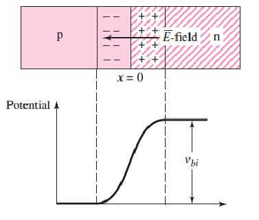
When the PN-junction is forward biased, current flows from P to N.
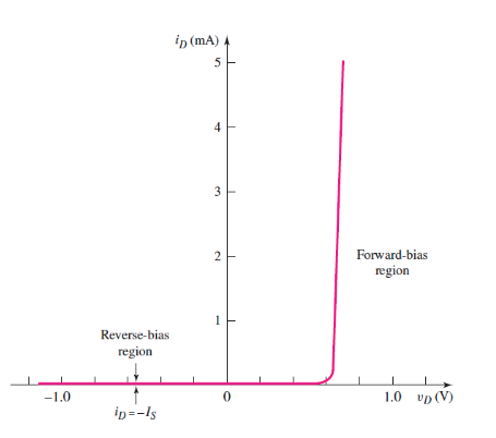
The PN-junction can be reverse biased too, and at a certain point ("the knee"), the bias will break down and current flow in reverse
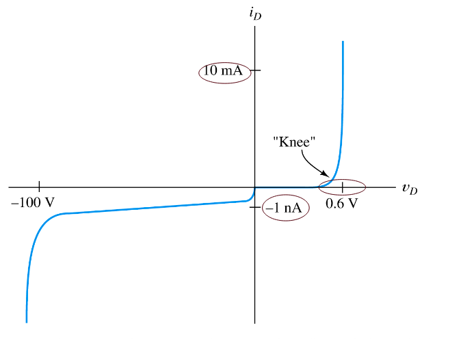
The graph shows a typical small-signal silicon diode at a temperature of 300k. Zener Diodes are diodes where the reverse breakdown voltage is controlled during manufacture to create diodes that act as voltage regulators when reverse biased.
The Shockley equation for a PN-junction related diode current and voltage :
Where I_s is the reverse saturation current, and is the thermal voltage. When v_D is large, typically :
Load Line Analysis
For the circuit below, KVL gives .
The Shockley equation also gives . Equating these gives a transcendental equation with no trivial solution.
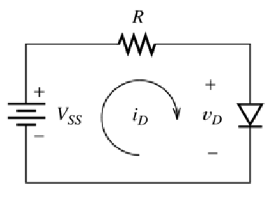
Instead, if an I-V curve is given, can perform load line analysis.
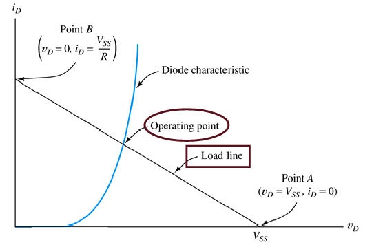
The load line is the straight line from one axis to the other, overlaid with the diode's I-V characteristic curve.
- Point B is a perfect short circuit, ,
- Point A is an open circuit, ,
The operating point, or Q (Quiescent)-point, is the point at which the two lines intersect, giving an operating point of .
If the diode is not conducting, then tiny to zero current flows. Otherwise, it will conduct almost perfectly at about 0.7 volts, so usually.
The Zener Diode
Zener diodes are designed to operate in the reverse breakdown region. The breakdown voltage is controlled by the doping level during manufacture, which allows a fixed voltage to appear between cathode and anode (that isn't just 0.7v). The ideal Zener diode behaves something like this:
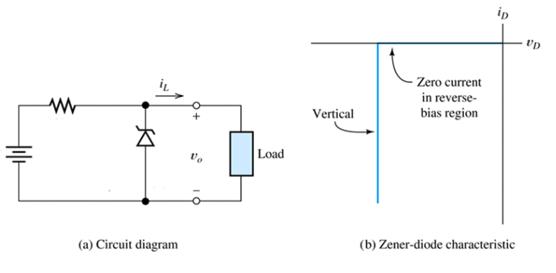
The circuit below shows a diode being used to regulate the voltage of a variable supply, to keep the voltage supply to a load constant
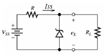
As an example, given a Zener diode's I-V curve, find the output voltage for and , with . KVL gives a load line of :
The graph shows the two load lines plotted with the diode I-V curve, giving of 10V and 10.5V, respectively.
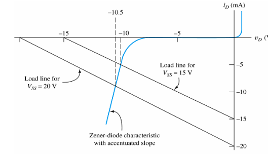
When modelling Zener diodes, an internal resistance is sometimes used, which is what gives the slope of the I-V curve as :
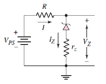
Oscillators
Oscillators employ feedback through amplifiers and frequency selective networks (capacitors/resistors) to create sinusoidal oscillation.
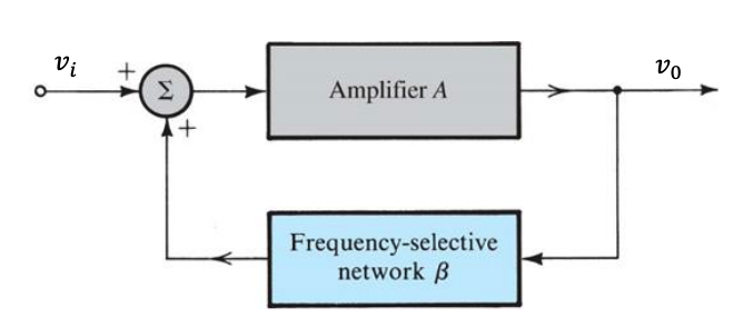
- is the closed loop gain of the system.
- is the open loop gain (with no feedback)
- is the feedback fraction, that feeds back a portion of the output voltage back to the input
- Negative feedback reduces the gain of the system, which is desirable because is often very large
- Stabilises circuits
- Reduces noise and distortion
- Increases bandwith
- Positive feedback is employed in the circuit above, which is how oscillators are built
- leads to oscillation
- Negative feedback reduces the gain of the system, which is desirable because is often very large
- Both positive and negative feedback are used in oscillators
- Loop gain is the gain just before the summing junction in the feedback
If at a specific frequency , the loop gain is unity, will tend to infinity. This is an oscillator. The condition for sinusoidal oscillations of frequency is:
At the phase of the loop gain must be zero and the magnitude of the loop gain must be unity. This is known as the Barkhausen criterion.
- The loop must produce and sustain an output with no input applied ()
- The frequency is determined by the phase characteristics of the feedback loop
- If loop gain , output grows
- If loop gain , output decays
It is difficult to get exactly unity loop gain. In terms of sinusoidal functions in the laplace domain, we are trying to place both the poles of the function on the imaginary axis in the s-plane. Poles in the right hand side of the plane will initiate oscillation, but bringing them back to the imaginary axis will reduce loop gain to unity and sustain oscillation. Poles in the left hand side of the plane will give a decaying sinusoid.
Wien-Bridge Oscillator
A Wien Bridge employs frequency selective positive feedback through the capacitor/resistor connected to the non-inverting op-amp terminal, and frequency independent negative feedback connected to the inverting op-amp terminal.
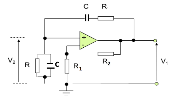
- is the open loop gain
- is the loop gain
For oscillation, we require , as this gives closed loop gain , which causes oscillation.
First analysing the positive feedback network in the laplace domain (capacitor has capacitance in the s-domain)
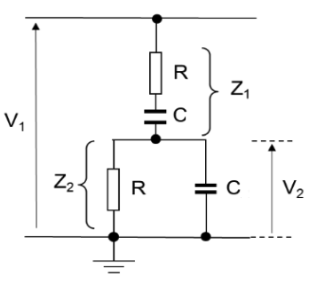
This is a frequency-dependant potential divider, so:
This is the transfer function of the frequency-selective positive feedback, as a function of . We require for a sinusoid, so:
The fraction above is real when , so:
Which gives:
The gain loss of the positive feedback network is when
As the feedback fraction , we require that for unity gain. The negative feedback circuit with the two resistors forms a non-inverting amp, so:
Verifying this using the overall loop gain:
Phase Shift Oscillator
A phase shift oscillator relies on 180 degrees of phase shift from inverting op-amp A3, and then 3 lots of 60 degrees of additional phase shift from 3 voltage-buffered RC networks. With 360 degrees of phase shift around the loop, the final stage gain is set such that

- The unity gain buffers provide voltage isolation between RC stages so the voltages
- Buffers have high input impedance and low output impedance, isolating stages to simplify analysis
- The maximum phase shift an RC network can provide is 90 degrees, but it is hard to achieve this so three 60 degree networks are used instead
- The final op-amp A3 creates a non inverting amplifier using and to give 180 degrees of phase shift
For 60 degrees of phase shift in an RC network, we require:
At the RC network also acts as a high pass filter, there will be a gain loss through them.
Using :
The gain loss for one RC stage is 0.5, so the 3 stages has a gain loss of . The inverting op-amp therefore must have a gain of -8 to give overall unity gain.
So the value of must be set accordingly.
Bipolar Junction Transistors
There are two kinds of BJTs, NPN and PNP. Both have a base, collector, and emitter and consist of two PN-junctions.
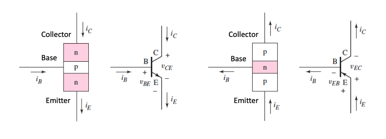
The operating mode of a BJT depends on how the junctions are biased.
- Forward active mode is used for amplification
- Cutoff and saturation modes are used for switching in digital circuits
- Cutoff is when both junctions are fully off
- Saturation is when both junctions are fully on
| Mode | Base-Emitter Bias | Collector-Base Bias |
|---|---|---|
| Cutoff | Reverse | Reverse |
| Forward active | Forward | Reverse |
| Saturation | Forward | Forward |
Transistors obey KCL, so all currents entering a transistor must leave:
Transistors also have common-emitter current gain,
There is also the parameter , the common-base current gain:
is usually large, so
Large-Signal Model
BJTs operating in forward-active mode can be modelled as shown:
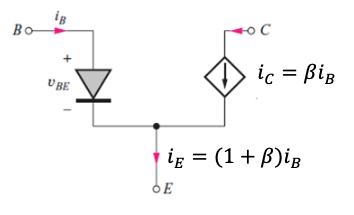
The current source shown is dependant upon the base current, and a diode is included to model the 0.7v drop across the PN-junction. This model assumes the transistor is biased correctly, as shown:
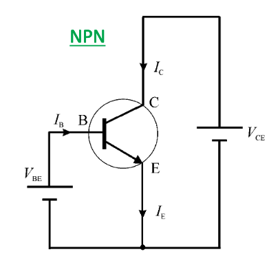
Biasing
Biasing is used to set up quiescent collector current to achieve optimum AC and DC conditions at the same time. is not well specified and can vary per device, so it should be designed to produce the correct operating conditions independent of device parameters and temperature. The Q-point is defined by and .
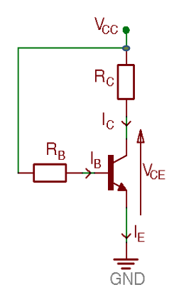
The circuit shows a single resistor base-biased circuit. Doing KVL around the base-emitter loop gives :
KVL between and ground gives :
Equations depending on are bad though, because can vary too much to rely on it as a parameter. The graph below shows the same circuit with the same resistors, as varies:
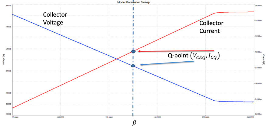
The Q-point shown is for , which gives and
Four-Resistor Voltage Divider Bias
This is the most widely used method to bias a BJT
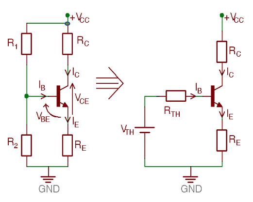
Thevenin's theorem is used to simplify the bias circuit
Applying KVL around the base-emitter loop:
As :
Therefore, the collector current :
Howere, we need to stabilise to not depend upon . If we choose to be small, ie , then we can disregard it along with :
The equation (approximately) no longer depends upon . Applying KVL around the collector-emitter loop for the voltage gives:
So, if is stable, then the Q-point is bias-stable. Stability is achieved through the choice of a small enough, , and also the inclusion of an emitter resistor which provides negative feedback stabilisation.
Compare the graph below with the same one further up for the single-resistor bias circuit. The voltage/current are much more stable and less dependant up on .
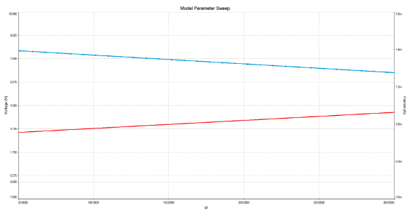
Transistors in Saturation
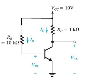
This can't be correct. The model breaks down as the transistor is saturated, its no longer operating in the forward-active region.
- The voltage accross the collector/emitter maxes out at about 0.2v
- The transistor then turns on like a switch
- Collector to emitter is (roughly) a short circuit
When operating in saturation, becomes :
This is much lower than a typical would be. As is increased further, decreases further and further.
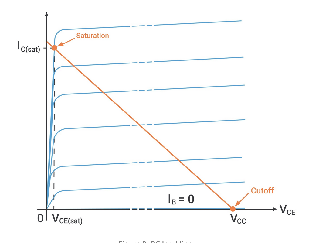
BJT Amplifiers
- BJTs make excellent amplifiers when biased in the forward-active region
- Transistors can provide high voltage, current and power gain
- DC biasing stabilises the operating point
- DC Q-point determines
- Small-signal parameters
- Voltage gain
- Input & output impedances
- Power consumption
- DC analysis finds the Q-point
- AC analysis with the small-signal model is used to analyse the amplifier
Hybrid-Pi Model
The hybrid-pi small signal model is what is used for hand analysis of BJTs:
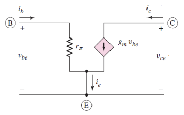
- Intrinsic low-frequency representation of a BJT
- Does not work for RF stuff
- Ignoring output impedance assumes is large
- Parameters are controlled by the Q-point
- Transconductance
- Thermal voltage
- Input resistance
For AC analysis, coupling capacitors are replaced by short circuits, and DC voltages replaced by short circuits to ground. The circuit below shows a 4-resistor bias amplifier replaced by it's small signal model.
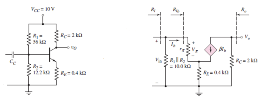
AC Analysis
The impdance at the base input :
The impedance at the emitter is reflected back to the base, multiplied by . This makes the overall input impedance of the amplifier:
The output impedance is easy, as lookong into the collector, we can see in parallel with a current source which has infinite impedance, so:
The voltage accross is the output voltage:
The voltage accross is the input voltage:
The overall voltage gain is therefore:
Note that the gain is negative meaning this is an inverting amplifier. If we make the assumption that , and that is large, then:
Common Collector Amplifier
The common collector (or emitter-follower) amplifier is another amplifier circuit used with BJTs (as oppose to the common emitter shown above).
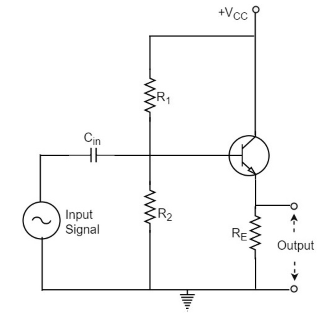
The hybrid-pi model of this circuit looks like, as without the collector the circuit can be re-arranged to:
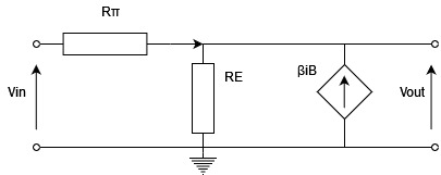
The output voltage is the voltage accross the emitter resistor, and as :
The input voltage is the voltage accross both the emitter resisitor and :
Therefore the voltage gain for this amplifier is:
As usually, , . This amplifier has very low voltage gain, and instead acts as a current amplifier:
The input impedance is large, as it is the reflected impedance from the emitter resistor again:
The output impedance can be calculate by shorting , and by applying a test current source accross the output terminals. I'm not going to type out all the analysis but:
The emitter follow has high input and low output impedance with a high current gain, so acts as an impedance transformer and a buffer.
Example
A circuit for a common-emitter amplifier is shown below.
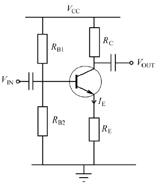
Work out the values of the DC biasing components , , and for the following conditions:
- Voltage accross
Assuming and , we have:
Calculating the Thevenin equivalent of the biasing resistors:
Then calculating the bias resistors from the Thevenin values:
To derive an expression for the voltage gain, need to replace the BJT by it's small signal model
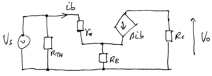
MOSFETs
Metal Oxide Semiconductor Field Effect Transistors are the dominant type of transistor nowadays, due to their simplicity to fabricate in VLSI applications. They are voltage controlled current sources, unlike BJTs, which are current-controlled.
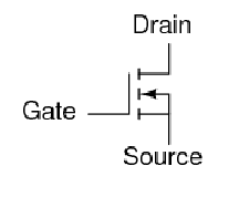
- By convention, the source terminal is at lower voltage than drain, so
- MOSFETs have three regions of operation
- Cutoff
- Linear
- Saturation
- Different to BJT saturation
A MOS transistor is characterised by it's transconductance:
Operating Regions
In the linear region:
- is the transconductance constant, a function of the semiconductor physics and geometry, and will be given.
- is the N-channel threshold voltage for the MOSFET
In this region, the relationship betwen and is (mostly) linear. The graph below shows the the current set by different voltages for different values of . The current begins to saturate at higher voltages, but is linear at lower values.
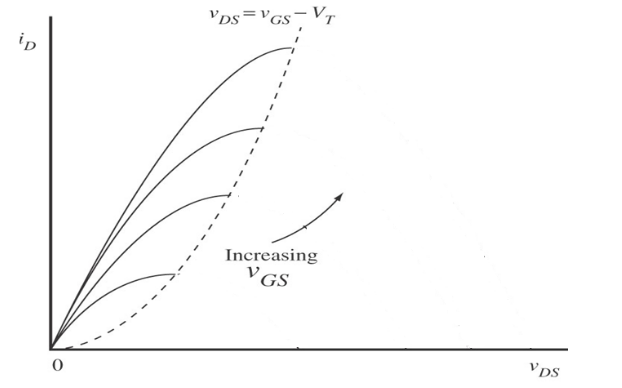
When operating in saturation, the drain current begins to saturate when:
in saturation:
In the cutoff region, no current flows, as .
- The saturation voltage
- Device is in saturation when
- Device is in linear region when
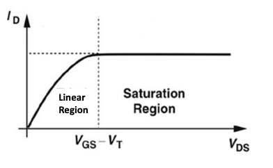
MOSFET Bias Networks
MOSFETs are useful in amplifiers when operating in saturation, when drain current is a function of gate-source voltage. As there is no gate current in a MOSFET:
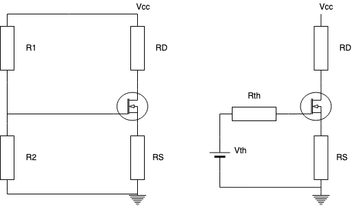
KVL around the gate-source loop:
Combinging this equation with gives the following quadratic equation in :
As the equation for drain current is quadratic, there are two possible solutions:
Only one of the solutions will be valid, so both must be calculated and checked. Using the following values:
Gives or . Checking the first one:
is a valid solution as , and .
Doing the same calculations for the other value yields a gate-source voltage that is below the threshold voltage, so the transistor is not operating in saturation and not conducting, meaning it can be disregarded.
MOSFET Amplifiers
Small-Signal Model
As MOSFETs have no gate current, their small signal model is much simpler than that of a BJT.

Between the gate and the source is an open circuit, but the voltage between the two sets the dependant current source . The MOSFET also has infinite input impedance.
Common-Source Amplifier
Similar to a BJT common emitter amplifier, can construct a MOSFET common source amp:
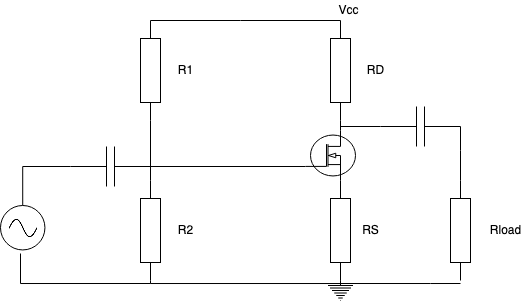
Using the small signal model of the MOSFET, this amplifier looks like this:
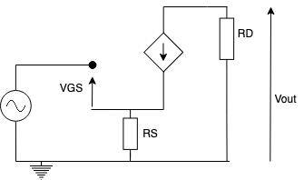
Drain current , so:
Note that transconductance in a MOSFET is:
This is much lower than transconductance in a BJT, hence the gain is much lower/
Bypass Capacitors
Adding a bypass capacitor to the amplifier increases the gain, while keeping the DC Q-point stable. Remember that capacitors act as short circuits in AC, and open circuits in DC.
The gain of the amplifier with a bypass capacitor is much higher.
Input and Output Impedance
- The input impedance of a MOSFET is infinite, as no current flows between gate and source.
- The overall input impedance of a common source MOSFET amp is , as the two gate bias resisisors will act as impedances to input signals
- The output impedance of the bypassed amplifier above is just , as that's the only impedance in the model.
- If , like in a common drain/source follower, then this becomes
- MOSFETs have higher input impedances for this reason, so MOSFET amplifiers are used over BJTs where high impedance is required.
Differential Amplifiers
Op-amps are differential amplifiers, designed to amplify the difference between two inputs. In an op-amp, the gain is usually very large, approaching in practice, and is modelled as infinite.
Op-amps are based on a circuit known as a long-tailed pair:
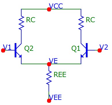
- and are a matched pair of transistors, meaning they have the exact same electrical properties (
- The quiescent current is the current through the shared emitter resistor,
- If is large, then
Biasing
When doing bias calculations, the two inputs and are assumed to be grounded, . As , . , the tail voltage, is always taken as negative. Using this, we can calculate :
sets the quiscent collector current.
When the two inputs are grounded, the output at the collectors and are the same.
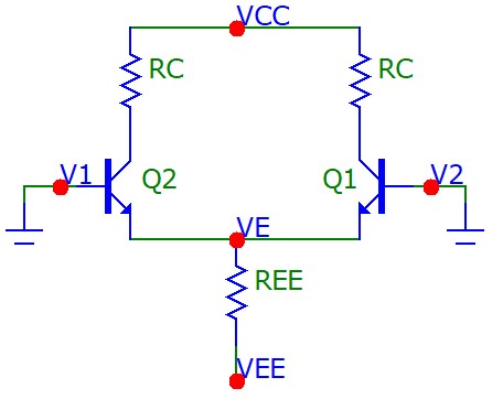
For matched transistors, .
AC Analysis
The long-tailed pair can operate in two modes, depending upon how input is applied
- Differential mode amplifies the difference between the two input signals
- Common mode works similar to a regular BJT amplifier
- Better amplifiers have a high ratio of differential to common gain, called the Common Mode Rejection Ratio (CMRR)
Differential Mode
The circuit below shows two AC sources connected, and , to give a differential input signal of .
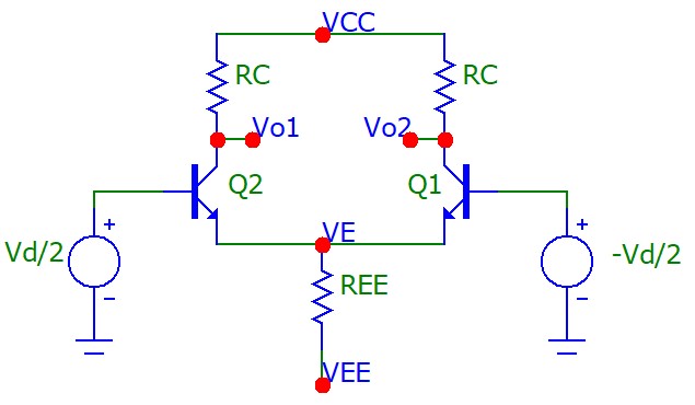
The differential output is the difference between the two outputs:
And the differential mode gain:
The way this circuit is usually used, however, is with one output referenced to ground:
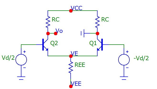
This gives a single-ended output, with a gain of:
The input and output resistances for differential mode inputs are:
Common Mode
Common mode input is when the same signal is connected to both input terminals, . An ideal differential amplifier would reject common mode input, but this is often not the case. The performance of a differential amplifier is defined by it's CMRR, which would ideally be infinite, but is usually just very large in practice.
The common mode input resistance:
The generalised output of a differential amplifier, factoring in both common mode and differential mode input signals is:
Example
Find to give , and for max AC swing, when .
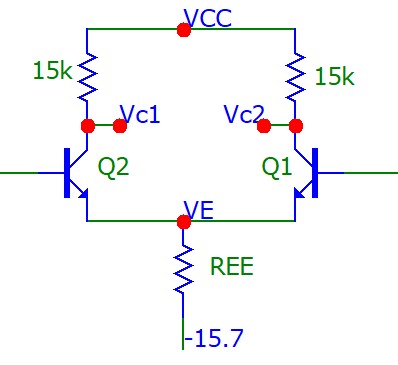
For max AC swing, :
Using , calculate the differential and common mode gains, and the CMRR of the circuit.
The common mode rejection ratio for this circuit is fairly low, because is low. as , so ideally is as large as possible. Replacing it with an ideal current source with infinite resistance can acheive this.
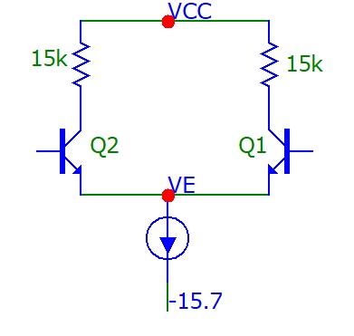
Op-Amps
Operational Amplifiers are fundamental to modern electronics

Properties of an ideal Op-Amp:
-
- Slew rate
- Output can change as fast as we want
- Common Mode Rejection Ratio (CMRR)
- Signals where are rejected and not amplified
- Power supply rejection ratio
- Bandwith
A large gain drives the differential input to zero , as the op-amp always tries to keep the two inputs the same.
Buffers
A buffer provides unity gain while acting as a signal buffer.
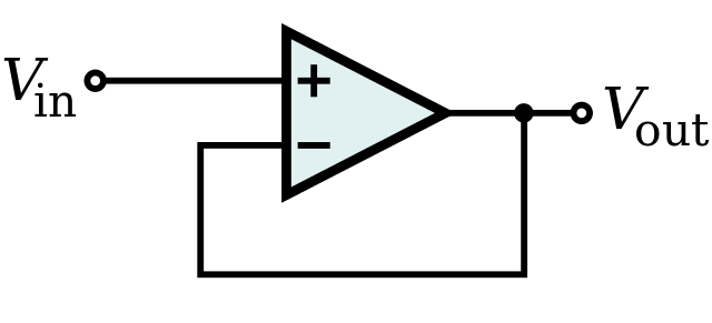
As is high and is low, no current flows in and there is no impedance to current flowing out, meaning the buffer acts to isolate stages of a circuit.
Active Filters
(they aren't really active, according to Ryan.)
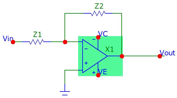
and are generalised impedances and can take any value. If , for example, then:
A limits test shows that this would make a low pass filter:
- As ,
- As ,
- The mid-band is where
Cutoff frequency is where , which is Hz
The other way round, where and is a high pass filter:
This gives a cutoff frequency of $f_c = \frac{1}{2 \pi R_1 C$, where the max gain as is
Equations
Below are some of the main equations that I have found useful to have on hand.
Use ./generateTables.sh ../src/es2c0/equations.md in the scripts folder.
| MOSFETs DC | |
|---|---|
| Stages | |
| Linear Region Drain Current | |
| Saturation Drain Current | |
| Saturation Drain Current -> VGS | |
| Small Signal Model | |
| Transconductance | |
| MOSFET Bias Network | |
| MOSFET input impedence |
| MOSFET Common Source | |
|---|---|
| Overall Input Impedence | |
| Overall Output Impedance | |
| Bypassed Gain | |
| Common Drain (Source Follower) | |
| Output Impedance |
Oscillators
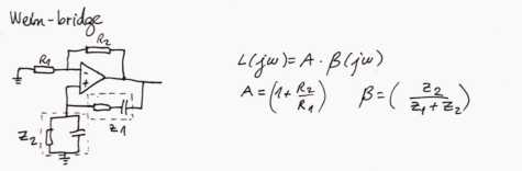
Closed Loop Gain
- is the closed loop gain of the system.
- is the open loop gain (with no feedback)
- is the feedback fraction, that feeds back a portion of the output voltage back to the input
Loop Gain
For oscillation, need unity gain, so angle therefore must be real, so also must be real.
Frequency Potential Divider ()
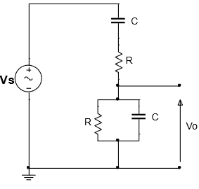
Frequency Potential Divider ()
Frequency of Unity Gain (0 phase shift)
60 Degrees of phase shift in CR network
Transfer function of CR Network
= Gain of CR network
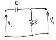
Transfer function of RC Network
= Gain of RC network
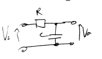
Transfer function of Inverse Frequency potential divider ()
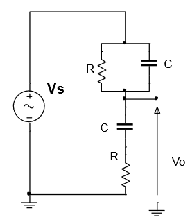
Transfer function of Inverse Frequency potential divider ()
Transfer function of Frequency potential divider (Inductor) ()
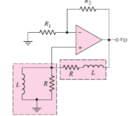
Transfer function of Frequency potential divider (Inductor) ()
Frequency of Unity Gain (0 phase shift) (Inductor)
BJT Transitors
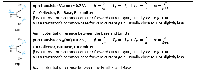
Common Emitter Forward Gain,
Common Base Forward current gain,
NPN Emitter Current
Emmitter Voltage Rule of Thumb
Thevin Resistance Rule of Thumb
Four Resistor Bias Circuit
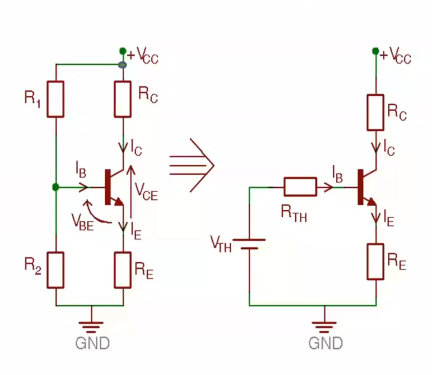
Four Resistor Bias Circuit
Transconductance
AC BJT Analysis
Amplifier Topologies
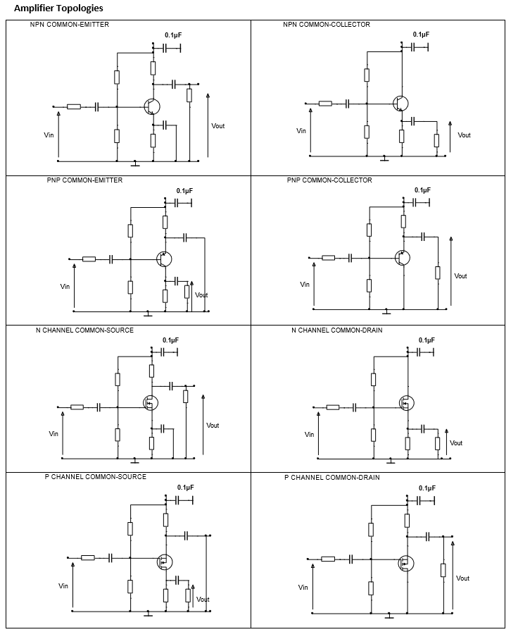
Transistor Input Impedance
Where = 25mV, = Collector current at Q point.
Gain of Collector Follower (Common Emitter) AC

Input Impedance of Collector Follower (Common Emitter)
Into the transistor
Output Impedance of Collector Follower (Common Emitter)
As current source has infinite impedance.
Emitter Follower (Common Collector)

- High Input, low ouput impedence
- High current gain
- So acts as impedence trasnformer and buffer
Voltage Gain of Emitter Follower (Common Collector)
as So low voltage gain, so instead current amplifier.
Current Gain of Emitter Follower (Common Collector)
Input Impedance of Emitter Follower (Common Collector)
Output Impedence of Emitter Follower (Common Collector)
Where = source input impedance
Output Impedence of Emitter Follower (Common Collector) Simple
Where = source input impedance
MOSFETs DC
No current through gate in MOSFET (as voltage controlled) (infinite input impedence)
Stages

- Cut off (no current flows,
- Linear
- Saturation
Where = Threshold Voltage
Linear Region Drain Current
, where = transconductance constant
Saturation Drain Current
Saturation Drain Current -> VGS
Small Signal Model

Transconductance
MOSFET Bias Network
Must check the two different values to see which ones are valid solutions.

MOSFET input impedence
As no current flows into gate
MOSFET Common Source
Similar to BJT common emmitter amplifier


Overall Input Impedence
As two gate bias resistors act as impedances to input signals. Therefore used over BJTs when high impedence required.
Is actually in parallel with source (input) impedence if it has it.
Overall Output Impedance
What the load resistor sees.
As current source has infinite impedence, therefore is the only impedence seen.
Unless there is an which would be in parallel with .
Bypassed Gain
Common Drain (Source Follower)
Output Impedance
Differential Amplifier
Long tail pair:
Modes Can operate in two modes.
- Differential (Amplfies Difference between two input signals)
- Common mode (Works similar to regular BJT amp)
Common Mode Same signal is connected to both input terminals.
- Ideal differential amp rejects common mode input, but not realistic
- Defined by CMRR
Better amps, have high ratio of differnetial to common gain, AKA Common Mode Rejection Ratio (CMRR).
Quiescent Current of Long Tail Pair
Current through shared emitter resistor, .
Biasing
and are grounded, therefore collector voltages are the same.
Collector Voltage of Grounded Long Tail Pair
And for matched transistors, .
Differential Gain without ground
Not really used
Differential Gain - Single Ended
Differential Input Resistance
Differential Output Resistance
Common Mode Gain
Common Mode Input Resistance
CMRR - Common Mode Rejection Ratio
Generalised Differential Amplifier Output
Both common mode and differential mode input signals are factored in.
Impedance Laplace
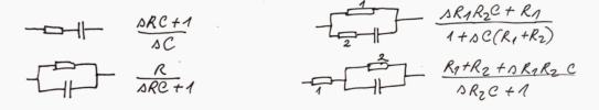
Resistor
Capacitor
Inductor
Resistor Capacitor Series
Resistor Capacitor Parallel
Resistor Inductor Series
Resistor Inductor Parallel
Op-Amps
Non-inverting Gain
Inverting Gain
Active Filter Gain
Active Filter Gain, Z2 = R2 || C
- Low Pass filter
- Cutoff where = Hz
Misc
Source Regulation
Fraction of change in load and input voltage
Load Regulation
Fraction of change in load to expected
ES2C6
Control Systems
- A control system contains processes with the purpose of obtaining a desired output given a specific input
- For example, consider a lift which rises from the ground to fourth floor:
- Pressing the button is a step input
- The lift rising is a transient response
- Two major performance measures
- Steady-state error
- Transient response
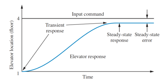
- Open loop control system configurations have an input that feeds directly into an output
- Cannot compensate for any disturbance
- Closed loop system feed the output signal back into the controller by subtracting it from the input
- Error drives controller to make corrections
General closed loop feedback control:
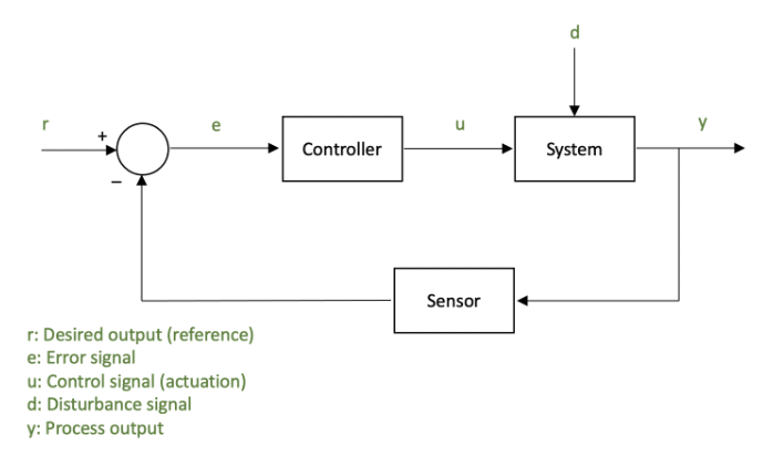
To design control systems, a system model is often needed. There are two general approaches:
- From first principles
- Uses known physical properties and laws (newton's laws, kirchhoff's laws, etc)
- Data-driven
- Identifies the system based on data collected
- Models usually take the form of a differential equation which describes the systems dynamics
- Used for simulation, control design, reference tracking, disturbance rejection, etc
Transfer Functions
Transfer functions give a ratio of output to input for a system.
Consider an th order linear differential equation, where is the output, the input, and and are the model parameters:
Taking laplace transforms an putting into a ratio of input over output:
![]()
- The transfer function of multiple systems
- Working with transfer functions is easier than ODEs as it they don't involve any differentials.
Example
Given the transfer function , find the response to a unit step input :
Transfer function of the step input , so:
Taking inverse laplace transforms:
Modelling
Two approaches to modelling a system:
- Physical modelling
- Data-driven modelling
Models are developed so we can obtain transfer functions for further system analysis. Focusing on mainly how to build physical models of systems from first principles, there are three main steps:
- Structuring the problem
- Intended use of the model
- Inputs/outputs
- Other parameters
- How do subsystems interact
- Draw a block diagram
- Formulate the basic equations
- Describe relationships between variables
- Write down conservation laws
- Write down relevant relationships
- Formulate the ODE
- Express time derivatives of relevant variables
- Express outputs as function of inputs
There are two main physical systems relevant to this module, electrical, and rotational mechanical. The properties of the main components of these systems are shown in the tables below:
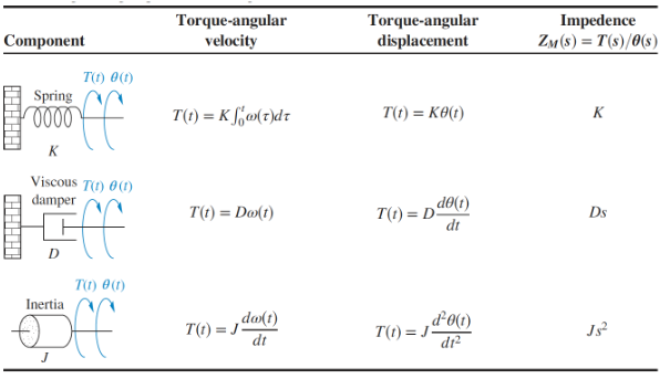
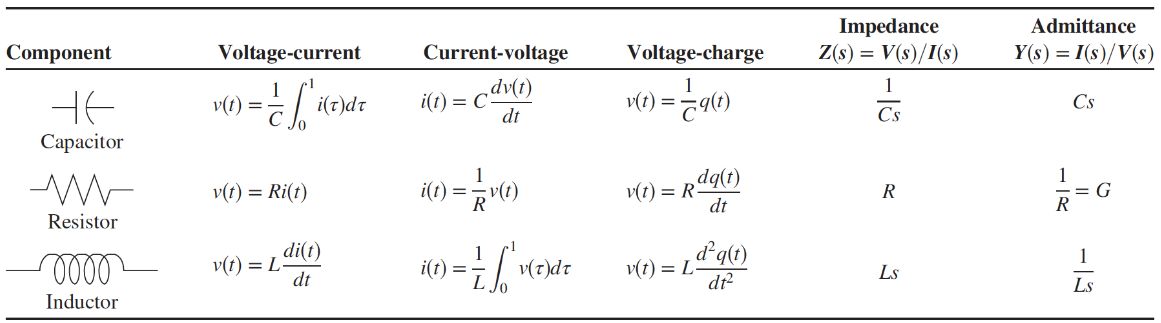
Rotational Systems
In a rotational system, we are interested in the relationship between applied torque and angular displacement. The sum of the applied torque is the sum of the moments of all the components. For example, obtain the equations of motion for the system shown:
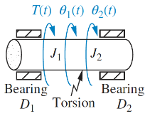
The system has an input torque at , two inertias and , the two bearings act as dampers and , and the torsion acts as a spring :
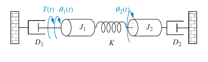
For inertia :
And for :
Note that for both these equations the form is [sum of impedances connected to motion] - [sum of impedance between motions] = [sum of applied torque at motion]. This general form can be applied to any rotational (or electrical) modelling problem.
Electrial Systems
Obtain the voltage-current relationship of the following electrical system:
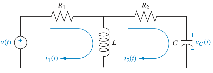
Using KVL for loop 1:
And loop 2:
Again, noting that the form of the equation is the same as rotational: [sum of impedances around loop] - [sum of impedance between loops] = [sum of applied voltage]
Block Diagram Algebra
A subsystem can be represented as a block with an input,output, and transfer function. Multiple blocks are connected to form systems, which involve summing junctions and pickoff points:

There are a few familiar forms that always pop up in block diagrams, that can be reduced down into simpler blocks:
Cascade Form
In a cascade form, each signal is the product of the input and the transfer function. The transfer functions of blocks in a cascade are multiplied to form a single function.
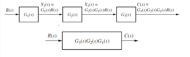
Parallel Form
In a parallel form, there is a single input, and the output is the sum of the outputs of all the subsystems.
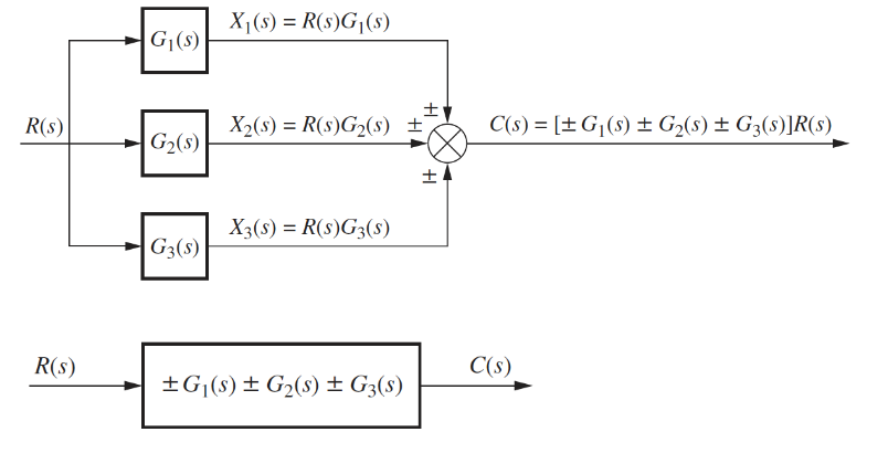
Feedback Form
Feedback form is the most important form encountered in control systems:
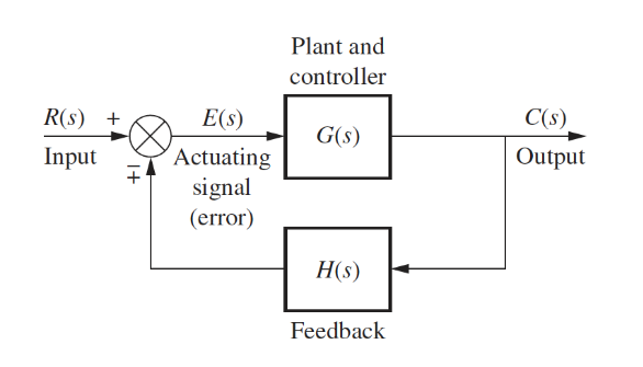
This can be reduced to a single transfer function:
Other Identities
Moving left past a summing junction:
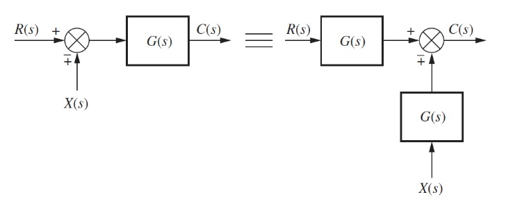
Moving right past a summing junction:
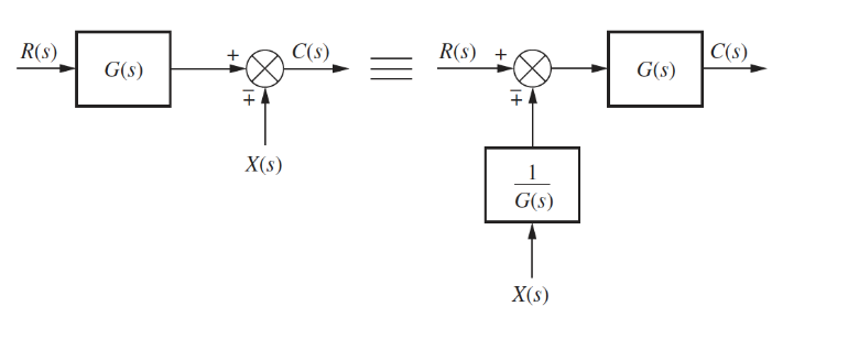
Moving left past a pickoff point:
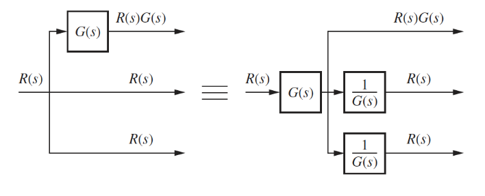
Moving right past a pickoff point:
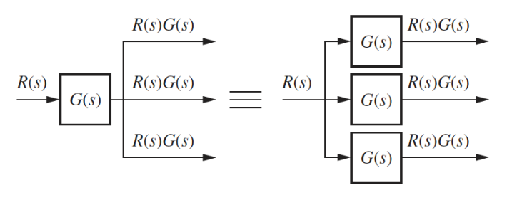
Example
The goal is to rearrange diagrams into familiar forms that can then be collapsed
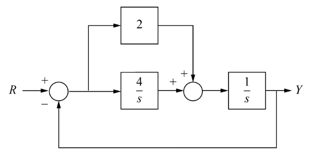
Forming the equivalent parallel system:
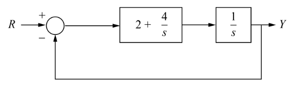
Collapsing the cascade:
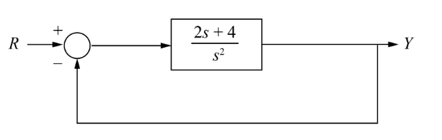
We now have a single transfer function that is the ratio of output/input for the entire system.
Poles and Zeros
A system can be analysed to obtain time response characteristics
- Transient response is the initial response that takes place over a time before reaching steady state
- Steady state response is the final response of the system after the transient has diminished
Conside the general form of the transfer function:
- Poles are the roots of the denominator
- The values of that make infinite
- Zeros are the roots of the numerator
- The values of that make zero
As is a complex number, poles and zeros can be plotted on an argand diagram. If , then the transfer function has a pole at and a zero at :
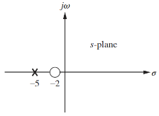
To further analyse this transfer function, we can give it an input step to analyse it's step response. The overall transfer function is now given by:
This shows that:
- The pole of the input function generates the form of the forced response (constant term)
- Step input has a pole at the origin, which generates a step function at the output
- The pole of the transfer function generates the form of the natural response
- gave the form
- The pole of the real axis generates an exponential response of the form
- The farther to the left a pole is, the faster the transient decays
- Poles to the right of the imaginary axis will generate unstable responses
- Zeros and poles generate amplitudes for both forced and natural responses
Stability
- Stability is the most system specification in control design
- Unstable systems are useless
- The definition of stability used here is that of a linear time invariant system
- Any that can be represented as a transfer function
The response of any system can be expressed as the sum of it's forced and natural responses:
- A system is stable if the natural response decays to zero as
- A system is unstable if the natural response grows without bound () as
- A system is marginally stable if the response is constant or oscillatory
The stability of a system is defined by the poles of it's closed loop transfer function:
- If the poles are all negative, the system is stable and decays exponentially
- An unstable system has at least one negative pole
- If a pole lies on the imaginary axis then the system is oscillatory
Transient Response Characteristics
The output response of a system for any given input depends on it's order. First and second order systems respond differently to the same input.
First Order
A first order system only has one pole. A general first order system with one pole and no zeros, subject to a unit step response:
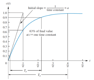
Note that there is only a single parameter, that describes the dynamics of this system.
- When , then
- This is the time constant, of the system
- The time it takes for the step response to rise to 63% if it's final value
- The further the pole from the imaginary axis, the faster the transient response and the lower the time constant
- Rise time is the time for the response to go from 10% to 90%
- Settling time is the time for the response to reach, and stay within, 2% of it's final value
Often it is not possible to obtain the transfer function of a system analytically, so we can obtain a time constant and other system parameters from data/graphs. The graph below shows a first order step response:
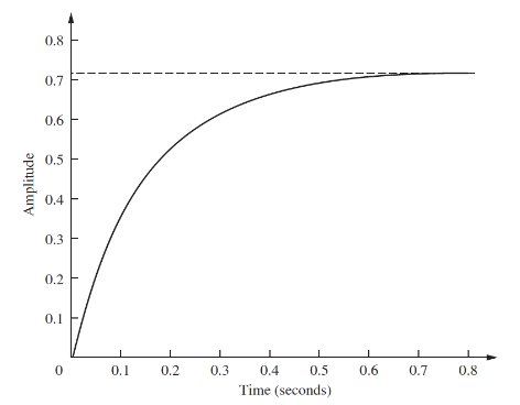
The final value of the response is 0.72, so the time constant is where the response reaches roughly , which is at about 0.13s. Hence . To find , we can use the final value theorem:
Second Order
A second order system exhibits a wider range of responses than first order. A change in parameter changes the shape of the response entirely. There are four kinds of 2nd order response:
Overdamped response has two poles and , both on the real axis, which exhibit the combined exponential response of the two poles.
Underdamped response has a conjugate pair of complex poles , with the real part exhibiting exponential response, and the imaginary part sinusoidal.
Undamped response has two imaginary poles, , exhibiting purely sinusoidal response.
Critically damped response has two repeated real poles, , so exhibits an exponential response, and an exponential response multiplied by time:
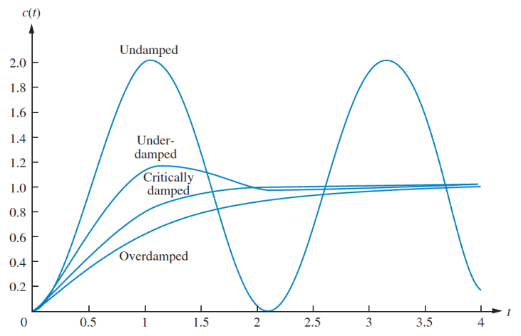
There are two other meaningful parameters of a 2nd order response:
- Natural frequency is the frequency of oscillation of the system with no damping
- Damping ratio is the ratio of exponential decay frequency to natural frequency
A general 2nd order transfer function is given by:
The damping ratio determines the characteristics of the system response:
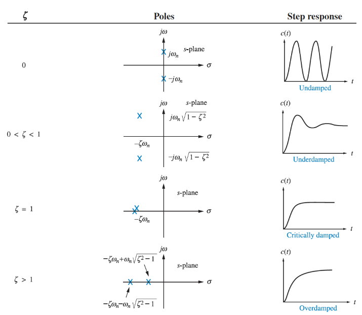
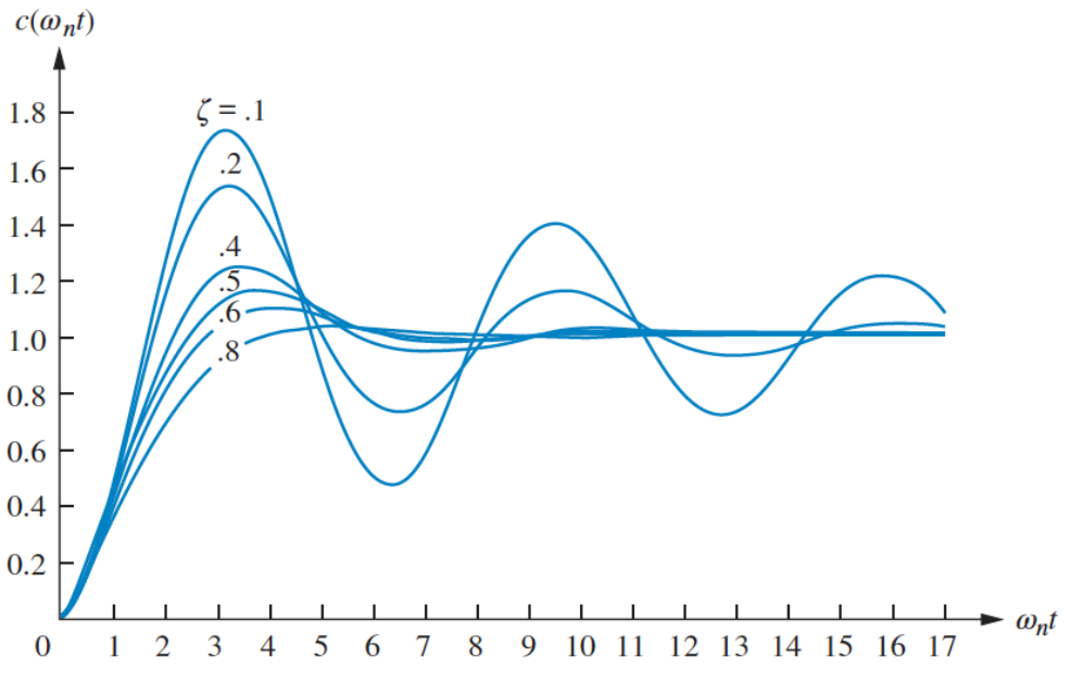
There are additional metrics that describe the response:
- Settling time
- Peak time is the time required to reach the first or maximum peak of the response
- Percentage overshoot % is the amount that the response overshoots the steady state value at it's peak, expressed as a percentage of the steady state value
- Rise time cannot be trivially defined for a 2nd order system
The damping ratio can also be defined in terms of these parameters:
Example
Find the damping ratio, natural frequency, damping characteristics, peak time, overshoot, settling time of:
As , this is an underdamped system.
Steady State Response Characteristics
Steady state response is the final response of the system after the transient has diminished. The primary design focus with control systems is around reducing steady state error, the difference between the input and the output (). In the graph below, output 1 has zero error, while output 2 has finite steady state error. It is possible for a system to have infinite steady state error if it continues to diverge from the input.
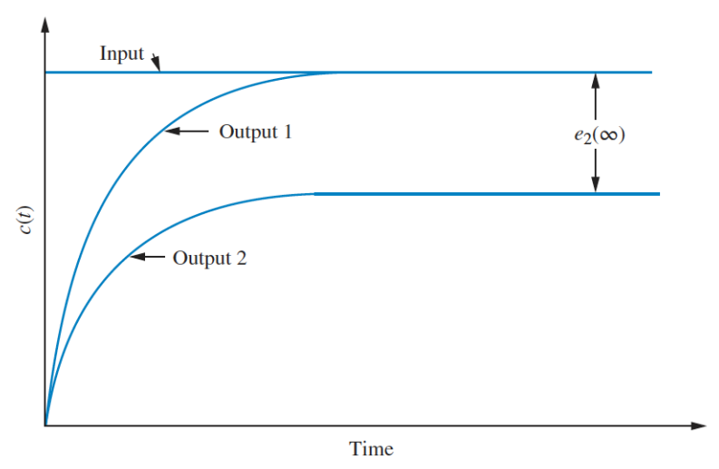
For three different kinds of test input, the corresponding steady state errors are given as
Step input:
Ramp input:
Parabolic input:
,, and are static error constants associated with different input types.
In order to acheive zero steady state error for a step input the denominator of has to be 0 as , which is only possible if in the equation below:
Meaning that there must be at least one pure integrator (multiple of ) present in . For ramp and parabolic input, the same applies for and .
PID Controllers
PID controllers are a control method that consits of a proportional, integral, and derivative of an error input :
PID controllers are widely used as they are robust, versatile, and easy to tune. The tuning parameters are the three constants, , , and
- Increasing the proportional term increases the output for the same level of error
- Causes the controller to react harder to errors so will react more quickly but overshoot more
- Reduces steady-state error
- The inclusion of an integrator helps to eliminate steady-state error
- If there is a persistent error the integrator builds and increases the control signal to reduce the error
- Can make the system respond slower and be more oscillatory
- The derivative term allows the controller to anticipate error
- The control signal can become large if the error is sloping steeply upwards, irrelevant of magnitude
- Adds damping to the system to decrease overshoot
- Does not affect steady-state error
| Rise time | Overshoot | Settling time | Steady-state error | |
|---|---|---|---|---|
| Decrease | Increase | Small change | Decrease | |
| Decrease | Increase | Increase | Decrease | |
| Small change | Decrease | Decrease | No change |
PID Tuning
Tuning a PID controller can be done easily if a model of the system can be derived, as then analytical techniques can be applied to determine the ideal parameters. If a model cannot be obtained, then an experimental approach is required. The Ziegler-Nichols method is one common approach. The three constants are determined based upon the transient response characteristics of a given system, and there are two different methods, both aiming to give less than 25% overshoot.
Note that for the Ziegler-Nichols method, integral and derivative gains are used, where and
- The first method involves experimentally obtaining a unit step input
- If the system involved neither an integrator, or dominant complex poles then the output will look like an s-shaped curve
- This is when this method applies
- If this method doesn't apply, the system likely has a built in integrator, and the 2nd method is needed
- The curve is characterised by two parameters, the delay time and time constant :
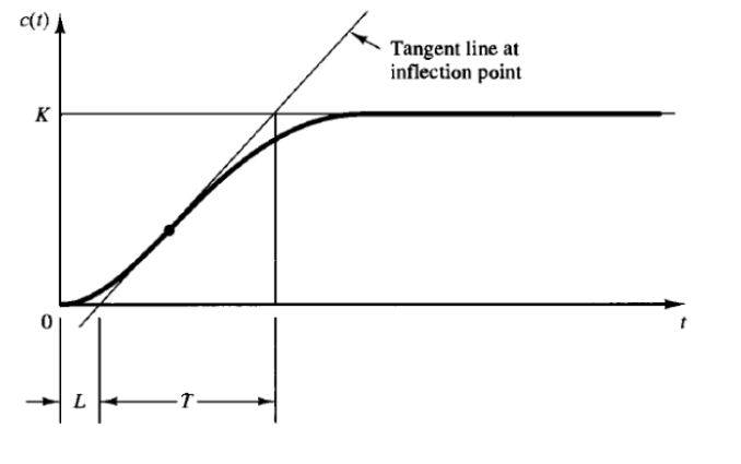
The transfer function can then be approximated by:
And the PID constants are set according to the following:
| Controller type | |||
|---|---|---|---|
| P | 0 | ||
| PI | 0 | ||
| PID |
For the second method:
- Set and . Using only
- Increase the constant to a critical value at which the output exhibits sustained oscillation
- If this does not happen for any , this method is not applicable
- The critical gain, and corresponding critical oscillation period are experimentally determined
- These are then used to set the other constants as per the following:
| Controller type | |||
|---|---|---|---|
| P | 0 | ||
| PI | 0 | ||
| PID |
Sometimes further tuning is required beyond these two methods to fine-tune the parameters to gain a response suitable to the application.
Drive Systems
Rotary Systems
- A rotary system is a system in which the load is rotating
- A direct drive system is one in which the motor is directly driving a load through a shaft
- No other transmission system other than the shaft
- All components have the same angular velocity
- Inertia is the rotary equivalent of mass
- Torque is the rotary equivalent of force.
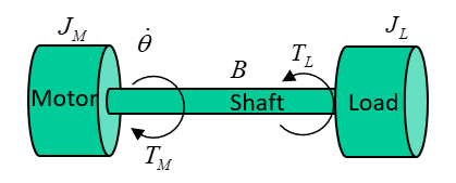
System parameters:
- = motor inertia, kgm
- = load inertia, kgm
- = torque load, Nm
- = motor torque, Nm
- = shaft damping, Nm/rad/s
- = angular velocity, rad/s
The system equation for how much torque the motor must provide is:
The system's total moment of inertia is the sum of the inertias in the transmission system and load referred to the motor shaft, plus the inertia of the motor.
- The inertias here can be summed as the have the same angular velocity
- The load will accelerate or decelerate depending on whether the applied torque is greater than or less than the required driving torque
- For an accelerating system, the motor must overcome thr torque load, frictional forces, and the total inertia of the system
- For a decelerating system, the frictional forces and torque load work to slow system down, but system inertia must still be overcome
Example
Using the same system shown above with parameters:
To rotate the load from stationary to 20 rad/s, at an acceleration of 10 rad/s, the torque delivered is:
- Nm at
- Nm at
- Nm at
- It can be seen that for a given motion trajectory, the maximum torque load was when the system was still accelerating, but had reached its final velocity
- Decreasing the acceleration will reduce the maximum torque requirement, which will reduce load on the motor
- More torque is required to accelerate a load than decelerate it due to friction
- If there is a torque load remaining when the load is stationary, the motor must compensate for this
Moments of Inertia
An object's moment of inertia is determined by it's shape, and the axis through which it rotates. For a point mass the moment of inertia , where is the mass and the perpendicular distance from the center of mass to the axis. Infinite infinitesimally small masses can be considered to calculate the moment of inertia of an entire body through integration.
Fortunately, this is rarely needed as the inertias of common shapes through all 3 axes are given:
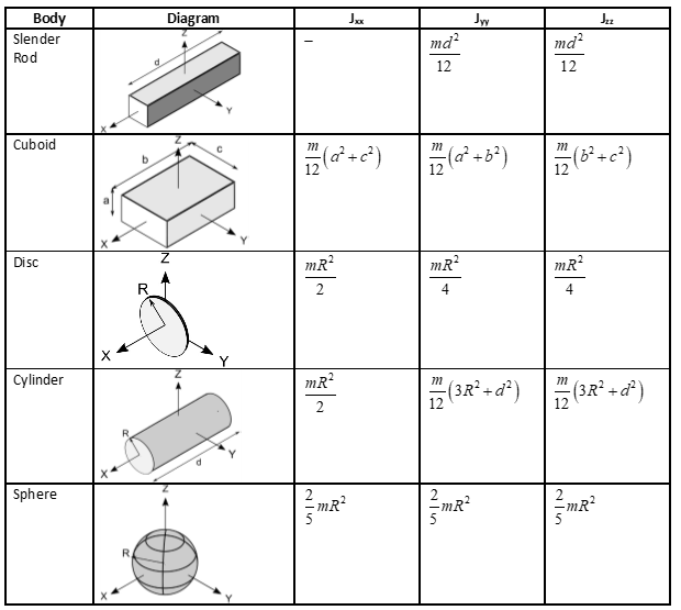
For rotation about an axis other than one through the centre of gravity, the parallel axis theorem can be used. The parallel axis theorem states that the moment of inertia about any axis is equal to the moment of inertia about an parallel axis through the centre of gravity , plus the mass of the body times the square distance between the two axes :
Example 1
The body shown is modelled as two 30kg spheres with radii 0.1m, connected with a slender rod of length 1m with weight 10kg. The whole body rotates about the axis, shown. Calculate the total inertia.
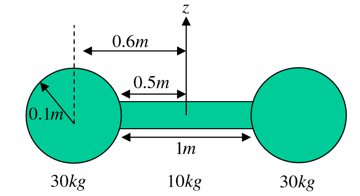
First the moment of inertia of the rod about the axis:
The moment of inertia of the spheres requires the parallel axis theorem:
Total inertia:
Example 2
Derive an equation for motor torque in the system below
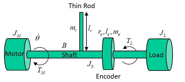
- Rod length
- Rod mass
- Encoder radius
- Encoder length
- Encoder mass
- Shaft radius
Inertia of encoder:
Inertia of rod using the parallel axis theorem, with the axis through it's centre of mass halfway up it's length parallel to the shaft:
The total inertia:
Deriving the equation for motor torque and then substituting in:
Geared Rotary Systems
Connecting a load to a motor via a gearbox allows a motor to drive higher torque loads, at the expense of reducing the angular velocity (or vice versa). Analysis of such systems is more complex as there are different velocities involved. Systems can be reduced to an equivalent direct drive system by referring torques accross the gearbox.
- Assuming a gearbox is 100% efficient, input and output power are the same
- Angular velocity is decreased and torque increased by a factor of
- If , the inverse happens
- The gear ratio is defined as the number of teeth on output gear over the number of teeth on the input gear
- The sign of the output is determined by the structure of the gearbox, two gears will rotate in opposite directions
- Three gears in chain will rotate in the same direction
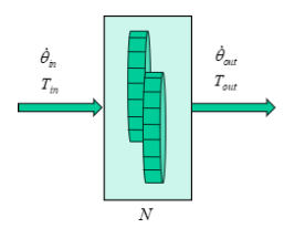
In general, terms reflected across a gear system are:
Example 1
A geared rotary system is shown below. Derive an equation for the torque delivered by the motor
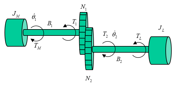
Total inertia is the motor inertia plus the load inertia reflected across the gearbox
Reflecting the damping and torque load too:
Final equation:
Gear Ratios
The chosen gear ratio affects the behaviour of the system, so the gear ratio is an important design choice. Minimising the peak torque requirement of the motor is important and can be done through the gear ratio.
In the example above, the peak torque when accelerating to 20 rad/s at 10 rad/s is 0.48 Nm. This is still less than direct drive, but there is an optimal gear ratio that minimises the strain on the motor. Through differentiation, this is found to be:
The minimum torque in a geared assembly with no torque load is achieved when the reflected load inertia is equal to the motor inertia. There are a few reasons why this may not be achevied, however:
- The term also must include additional components such as encoders, couplings, etc, each of which require energy input which is not then available to the load
- The gears also have an inertia which represents a loss factor as torque is required to turn these
- Off the shelf gears come in finite configurations so there may not be available components which match the theoretical optimum
Gear ratios may also be optimised to reduce the angular velocity and power of the motor, which may be a more desirable outcome. In practice, either acceleration or torque will be optimised for, or a compromise between the two must be made.
Example 2
For the geared system with a torque load shown below, find the gear ratio that minimises the torque delivered by the motor

The motor torque is the acceleration times total inertia, plus referred torque load
Rearranging for acceleration:
The addition of a constant torque load changes the optimal gear ratio, which is now given by:
This is the optimal gear ratio for a geared rotary system with a constant torque load
Torque Loads
There are 4 main types of torque loads:
- Windage torque
- Motor is driving a component that moves fluid such as a propeller in water, or a fan
- Torque load is proportional to square of the speed of the motion
- Can be useful, such as a fan
- Can be considered a loss, such as a motor doing work to move air when it should be rotating a shaft
- Electromagnetic torque
- Exists in motors because that's how motors work
- If the same machine is being driven mechanically to generate electricity, ie in a generator, electromagnetic torque must be overcome
- is the EM torque generated from input electrical energy
- Resistive torque
- Any mechanical resistance to the torque, such as overcoming gravity by lifting a mass with a pulley
- Any resistive force seen by the motor as torque
- Frictional torque
- Any two moving surfaces in contact
- Two models of friction
- Coulomb friction
- Constant independent of velocity
- Coefficient multiplied by the sign of the velocity such that it always resists motion
- Viscous friction
- Coefficient multiplied by velocity
- Both models summed to give a more accurate frictional model
- Values of constants can be found experimentally
Motion Profiles
Most rotary and linear systems can be categorised as either:
- Incremental Motion
- Repetitive motion between two positions
- Time and distance are important
- Velocity is secondary
- For example, pick and place
- A conveyor belt that has stop/start behaviour
- Constant Motion
- Velocity and distance are more important
- A machining operation such as CNC milling
- A conveyor belt that reaches a fixed velocity and keeps going
There are four types of motion profiles:
- Triangular
- Trapezoidal (the only examinable one)
- Cosine
- Polynomial
They are defined by:
- Acceleration time
- The time spent at constant velocity, slew time
- Deceleration time
- Total motoring time
The beginning and ends of the time are dentoed and , where and are the beginning and end of the slew time.
Additionally, is a value whch is defined as the fraction of the total runtime for which velocity is constant:
Trapezoidal Motion
We want to define the acceleration, velocity, and position in the three distinct time periods: accelerating , constant velocity , and decelerating .
We can also define the time periods with respect to :
And the max velocity/acceleration:
Gearboxes
Rotary transmission systems (gearboxes) used multiple gears compounded together with intermediate shafts
- Driven gears are rotated by another gear
- Driver gears are rotated by a shaft
- Used where higher gear ratios are needed
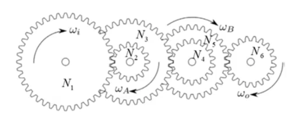
The gear ratio for compound gears like this:
- Gears 2,4,6 are driven gears
- Gears 1,3,5 are driver gears
Worm and Wheel
A worm and wheel gearbox changes the axis of rotation and provides a high gear ratio
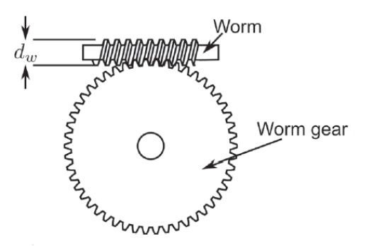
- The worm drives the wheel
- Wheel cannot drive worm
- The lead is the distance the worm moves forward in one revolution
- is teeth on worm, is axial pitch in meters
- The axial pitch is the distance between each thread on the worm gear
- A worm with one tooth is single start, two teeth double start, three teeth triple start
- Gear ratio is wheel teeth / worm teeth
- To drive the gearbox backwards,
- is coefficient of friction
- is angle formed by the triangle between the length of the worm , and
- is diameter of the worm gear
- In most applications , so cannot be drive backwards
Planetary Gearbox
A planetary gearbox is a co-axial gearbox, used in high-torque low-speed applications. It is cheap, compact, and efficient.
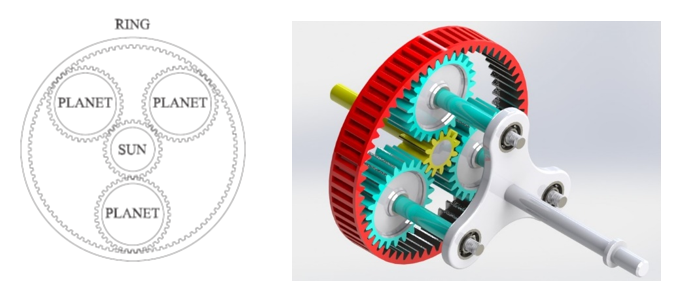
- Four main components
- Sun gear in the centre connected to one shaft
- Carrier connected to another shaft
- That fidget spinner-looking bit in the picture
- Outer ring
- Multiple planet gears connected to the carrier
- Relationship between input and output torque depends on which components are fixed in place
One of these velocities will always be zero, so the relationships are given below between velocities and torques for different fixed components
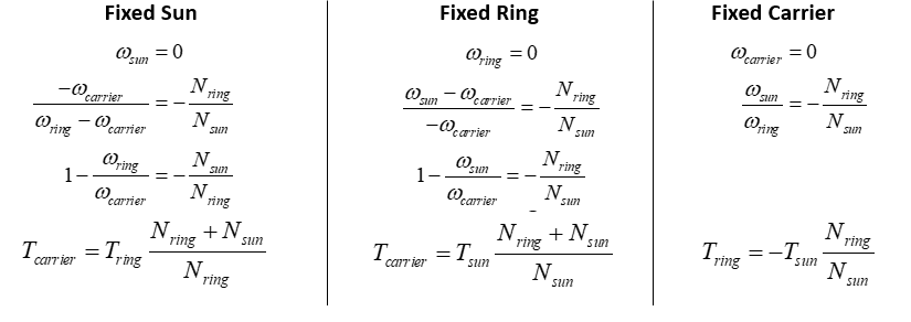
Choosing a Gearbox
An appropriate gearbox should be chosen based on velocities and torques in the system:
- Max intermittent and continuous velocities
- Max intermittent and continuous torques
- Gear ratio
- Radial and axial loads
Equivalent torque is found based upon the motion profile and average torques:
- is average torque in a time period
- is average velocity in a time period
- is a constant depending upon the gear construction, usually between 0.3 and 10
- Always use 5 here
Mean velocity is also required:
The selection process for an appropriate gearbox is as follows:
- Choose a gearbox whose maximum continuous torque (rated torque) is larger that
- Ensure max intermittent torque is frater than max torque load (torque at end of t_{acc})
- Divide the max gearbox speed by to determine maximum possible gear ratio
- Select a standard gear ratio below this value
- Input mean velocity is
- Input peak velocity is
- If either of these exceed gearbox velocity ratings, select a lower gear ratio and try again
Rotary to Linear Motion
Belt and Pulley
Transfers rotary motion across a distance
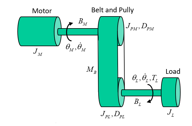
The rotational position, velocity, and acceleration of the motor and load are related by the relative diameters of the pulleys
The total intertia of the torque load is the intertia of the motor, pullets, belt, and load, all referred to the motor
The torque load must also be referred across the belt and pully system using the equation
The total torque the motor must provide for the belt and pully system shown is:
Lead and Screw
- The screw is rotated by the motor, which makes the nut move along the thread of the screw
- The distance the nut moves in one rotation is the lead
- The pitch is the distance between two adjacent threads
- The starts is the number of independent threads in a screw, typically 1-3
- The relationship between rotary velocity of the screw and linear velocity of the nut is
The diagram below shows a lead and screw subject to three forces
- Push-pull
- Gravity
- Frition
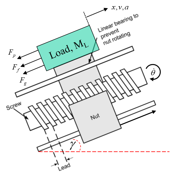
The forces must be referred to the motor as a torque, which is done using the lead
The equation above is written using lead in m/rev. Lead is sometimes given in m/rad, and the conversion is given as:
Conveyor Belt
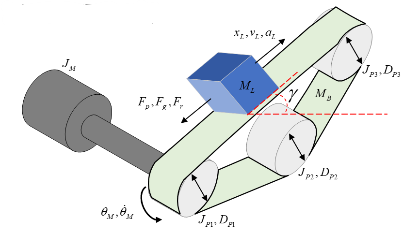
The position, velocity, and acceleration of the motor and the load can be related using the following formulae:
The inertia of each of the pulleys depends on their relative diameters, so the total intertia referred to each motor is it's own inertia, plus the intertia of each pulley, plus the load:
The forces from the load must be referred to the motor as a torque, which is done using the diameter of the pulley the motor is connected to also:
Rack and Pinion
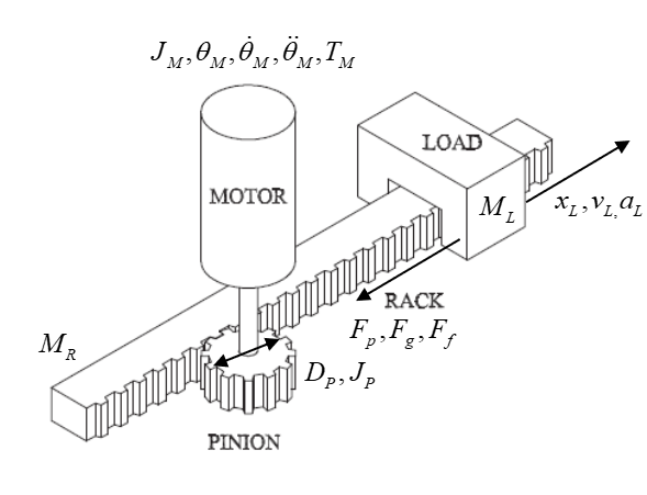
The equations for position, velocity, acceleration,inertia, and torque are literally all the same as for a conveyor what more do u want me to say
Transmission Efficiency and RMS Torque
- No gearboxes have 100% efficiency
- Efficiency modifies torque, not velocity
RMS torque is a useful metric of a system to inform the choice of motor used in design. Assuming a trapezoidal motion profile:
Sensors
Sensors measure physical quantities that are outputs from electromechanical systems. A sensed signal will go through a few steps before we have access to the data:
- The physical phenomena, the signal source, will happen
- The sensor will detect this by some mechanism and output a noisy signal
- Some signal conditioning/processing will take place to make the signal easier to read
- Analogue to Digital conversion samples and digitises the data
- The digitised data is presented to software as binary information
Performance of Sensors
There are a number of metrics used to measure the performance of a sensor, and which metrics are considered will depend upon the use case.
- Accuracy
- How close is the output to the true value of the input?
- A sensor with high accuracy will give readings close to the quantity being sensed
- Precision
- How consistent are the readings for the same input?
- How repeatable are the readings?
- Precise data is close to each other, but not necessarily to the true value
- High precision with low accuracy may be acceptable if the systematic inaccuracy can be compensated for
- Drift
- Changes in the output of the sensor not related to the input
- Often related to temperature, as this affects electrical properties
- Hysteresis
- The difference between the output when the input is increasing, and the output when the input is decreasing
- Quantities may be sensed differently depending upon their rate of change
- Common phenomenon and is often useful in other applications
- Often provided as an average percentage
- Linearity
- How the output changes with input over its operating range
- Linear behaviour is ideal as it simplifies output processing
- Many sensors have a linearity error of how much the output deviates from linear behaviour
- Resolution
- Changes in measured quantity may be too small to detect
- Sensor will have a max resolution which is the smallest changes it can sense
- Resolution also limited by ADC
- Gain
- How much the output changes with the input
- Too high and small changes will give large output swings and low noise tolerance
- Too low and the system will not respond to small changes
- Often given as how much voltage changes per measured unit
- A temperature sensor will have a gain in mV/°C
- Range
- The max and min values that can be sensed
- Can also define a linear range, the range for which the sensor has linear behaviour
- Can set a fixed operating range, to increase sensitivity or resolution over a smaller range
- Wider range usually gives lower sensitivity/resolution
Signal Conditioning
Generally sensor output is some voltage, which will be given as input to a microcontroller. Voltage signals can be too large, too small, or too noisy, so some conditioning/processing is required
- Filtering to remove noise
- Amplification to increase the range of the signal
- Attenuation to decrease the range of the signal
- Too large a voltage may damage the electronics
Op-amp circuits are usually involved in signal conditioning.
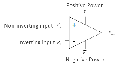
-
- is the open loop gain
- Both open loop gain and input resistance are in an ideal op amp
- No current flows in or out of the inputs
- The two inputs are always at the same voltage
Buffer
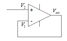
- The output is connected to the inverting input
- Negative feedback
- Provides decoupling between circuits
- No current flows into , but will still equal as the two inputs are always at the same voltage
- Ensures no current flows to provide protection
- No current is drawn from the supply by the op-amp
Comparator
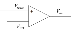
- Amplifies the difference between the two input voltages
- Output saturates at power rail voltages
- Useful for indicating when output reaches a threshold
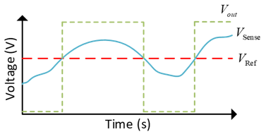
Inverting Op-Amp
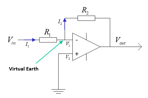
- Inverts and amplifies the input
- Amplifies small sensor output voltages
- (see ES191)
Non-Inverting Op-Amp
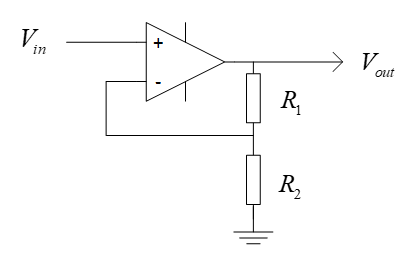
- Amplifies and does not invert input
Attenuation
Voltage attenuation can be easily achevied with just a voltage divider
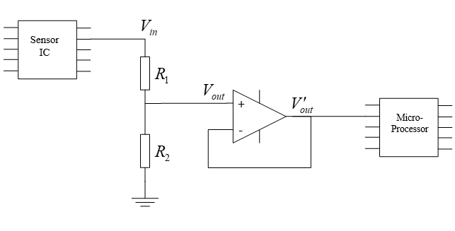
- has range 0 to 20V
- , ,
- has range 0 to 5V
Low Pass Filter
A low pass filter attenuates the high frequency components of a signal:
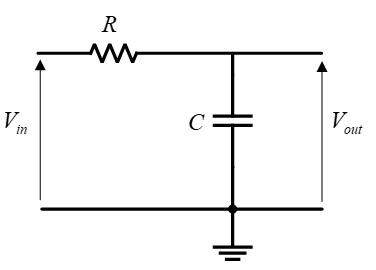
This is a voltage divider with a capacitor:
- The impedance of a capacitor is dependant upon frequency:
- Higher frequency, lower impedance
- The corner/cutoff frequency is where the output is -3 decibels smaller than the input (about 71%)
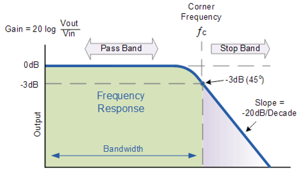
Reading Signals and ADC
- Signals are typically read with microcontrollers
- Input to microcontrollers has a maximum which if exceeded will damage the part
- Signals are read and digitised so they can be understood by digital electronics
- Signal is sampled at discrete time steps, at a sampling frequency
- Each sample is the value of the signal at time
- The sample value is held until the next sample, when the sample value is updated
- This creates a digital signal, an approximation to the input signal
- Sampling frequency has a large affect on how close the digital signal is to the original
- To maintain the highest frequency components of the signal
- is the highest frequency present in the signal, the nyquist frequency
- In practice, sample rate should be much higher than double
- Signal sample levels may only take a finite, discrete number of values
- Quantisation level
- Samples are rounded to nearest quantum
- Higher sampling resolution means more accurate digital signal
A signal measured with a 4-bit ADC:
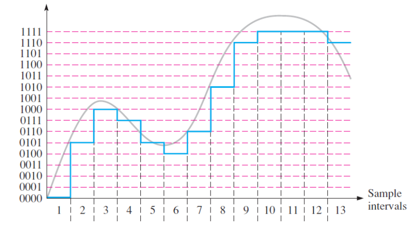
The circuit below shows a 3-bit ADC implemented with a priority encoder and op amps:
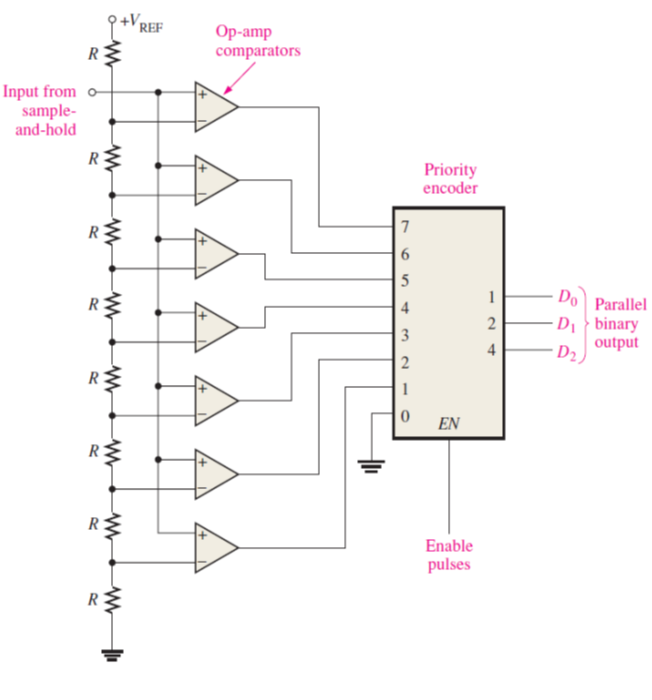
Wheatstone Bridge
A wheatsone bridge is a common circuit used to measure an unknown resistance:
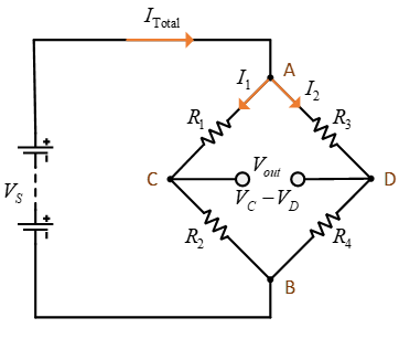
- 4 resistors, one with an unknown value
- Input is a known voltage
- Output is the measured difference between and
- Output of two potential dividers in parallel
- When , the bridge is balanced
This can be exploited to find the value of an unknown resistance. If , and is unknown and the rest are fixed values:
Can also derive an expression for in terms of the rest of the circuit, if is non-zero:
The unknown resistance may be some sensor which changes its resistance based upon a physical quantity, ie an LDR or strain gauge. The circuit below shows a photoresistor in a wheatstone bridge, with buffered outputs connected to a differential amplifier, which will provide an output voltage:
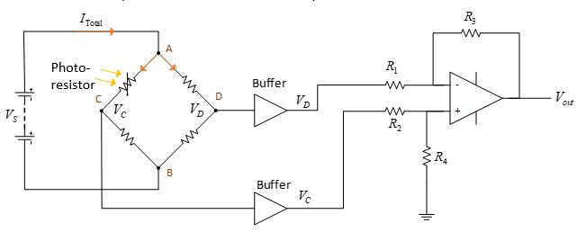
The gain of the differential amplifier is calculated using the following, where and
Force and Torque Sensors
Strain Gauge
- A thin strip of semiconductor which is wafer thin and can be stuck onto things
- The strip deforms as the surface deforms
- When subject to a strain, its resistance changes
- is the gauge factor, is the strain
- Strain is the ratio of change in length to original length, so this will measure how much a material has stretched by
- The diagram below shows how
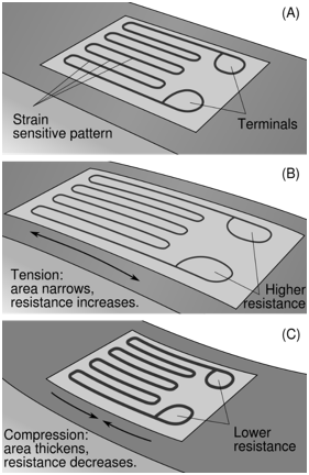
Load Cell
A load cell uses strain gauges to measure force:
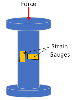
- As the force causes the shape to deform, the strain gauges sense this and the applied force can be calculated
- Important factors to consider are:
- Maximum force load
- How the force can be applied to the cell
- Rated output
Rotary Torque Sensor
Torque sensors work similar to load cells, using strain gauges to detect deformation.
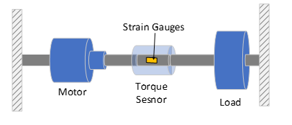
- The sensor is coupled to a rotating shaft
- The rotation of the shaft causes small deformations within the torque sensor, which are detected by strain gauges
Position and Speed Sensors
An encoder is a device that gives a digital output dependent upon linear or angular displacement.
- Incremental encoders detect changes in rotary postition from a starting point
- Absolute encoders give a rotational position
Incremental Encoder
- Incremental encodes contain a disc with multiple holes
- As the disc rotates, the holes will create pulses of light, with each pulse representing a displacement of a certain number of degrees
- Outer two layers slightly offset so direction of rotation can be determined
- Innermost hole counts number of revolutions
- The one shown has 12 holes so a 30° resolution

Absolute Encoder
- An absolute encoder works on a similar principal to an incremental encoder
- The output takes the form of binary code whose value is related to the absolute position of the disc
- Multiple layers used to provide unique encoding for each disc segment
- Encoders use gray coding so that if any holes are misaligned then error is minimised
- An 8-bit encoder has 360/256 = 1.4° resolution
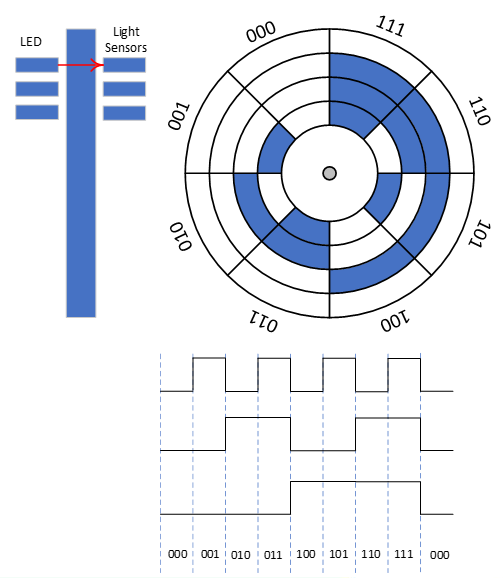
Speed sensors
- Encoders can also be used to measure angular velocity by measuring the time taken between pulses within the encoder
- Reflective photoelectric sensors work by reflecting light off a disc with reflective and matte colours, and measuring the rate at which the reflected light changes intensity
- Slotted photoelectric sensors work by detecting if a rotating part is blocking a beam of light or not
Current Sensors
Current Sense Resistors
- Due to Ohm's law, a current passing through a resistor will cause a voltage drop
- That voltage can be measured, and the current accross it calculated
- This will modify the voltage accross the load and cause a power drop
- A small resistor should be used, typically less than 10 ohms
Hall Effect Sensors
- Hall effect sensors use the physical phenomena of flowing electrons being deflected in a magnetic field to measure current
- A magnetic field will cause electrons to be deflected, which will charge either side of a sensor plate depending upon current direction
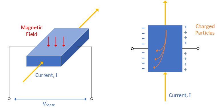
The potential difference between either side of the plate is given by
- is hall coefficient
- is the flux density of the magnetic field
- is current
- is plate thickness
Since , , and are constants, the relationship between current and voltage is linear.
Electromagnetics & Motors
There are 3 basic elements of any electrical machine
- Something to create a magnetic field on demand
- Something to channel said magnetic field
- Something to usefully be acted upon by the field
Magnetic Fields
- Magnets are dipoles, with a north and south seeking pole
- Moving charge creates a magnetic field
- A magnetic field is a region of influence where a force can act on a particle
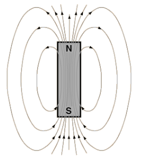
- Field lines are closed loops from north to south poles
- Lines never cross
- Closer the lines, stronger the field
- Lines are elastic, will always act to shorten themselves
Moving charges create a magnetic field, so a current moving through a wire will induce a magnetic field around the wire:
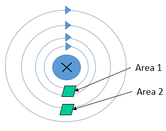
- The field radiates outwards from the wire
- Field is stronger close to the wire
- The number of field lines passing through an area is magnetic flux density , measure in Teslas
- Area 1 has a higher flux density than area 2
- The direction of the field is determined by the corkscrew rule
- Make a fist with your right hand
- Thumb is the current direction
- Fingers point in field direction
The magnetic flux density around a conductor is is calculated:
- is flux density in Teslas (T)
- is current in Amps (A)
- is the distance from the conductor in meters (m)
- is the permeability of free space in Henries per meter H/m
Flux density may also be expressed in terms of flux :
- is magnetic flux in Webers (Wb)
- is the enclosed area in square meters (m)
When there is more than one conducting wire, current in the same direction will augment a field
- A long wire with coils will create a solenoid
- Each extra turn develops a given flux, re-enforced with each turn
- The total flux available in a solenoid is the flux linkage in weber-turns
Permeability is a measure of how well a material builds a magnetic field under the influence of a magnetising source. A coil of turns carrying a current with length develops a magnetic field intensity , in amp-turns per meter:
The useful magnetic field from which is then
By using a material with higher magnetic permeability, we can create a higher magnetic flux density.
- Permeability is often given in terms of the permeability of free space, and the material's relative permeability:
- Ferromagnetic materials have high permeability
- Non-ferrous materials have low permeability
- Magnetic cores of ferrous materials are used in solenoids to channel the field
- An iron core has a higher permeability than air
- Stronger field creates a higher flux density
A current-carrying wire will interact with a magnetic field to create a force
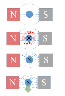
Fleming's left hand rule explains how this works, with force, magnetic field and current all acting in opposite directions.
A loop of wire in a field will have current flowing through it in opposite directions, so the wire will spin as equal forces will be induced on it in opposite directions. This is the basic principle behind how motors work.
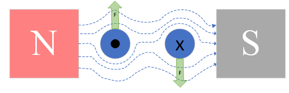
The force on a conductor in a magnetic field can be calculated:
- is the force on the conductor in Newtons (N)
- is the flux density in Teslas (T)
- is the current in Amps (A)
- is the wire length in meters (m)
- is the angle between the plane of the coil and the magnetic field lines
Magnetic Circuits
Magnetic circuits can be thought of in a similar way to electrical:
- Magneto-motive force causes flux to flow through various reluctances
- - Hopkinson's Law
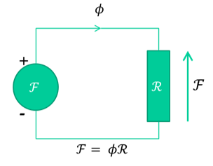
Magneto-motive force is considered the potential for a device to produce flux, and is related to the current and field intensity by:
- Flux is akin to magnetic current
- Reluctance defines how much flux a given potential develops
- Reluctance is a function of the geometry and material of the flux pathway
- Similar to electrical resistivity
Hysteresis/ B-H Curves
- The magnetic field obtained is a function of field intensity, the direction it is applied, and the existing field
- Saturation is the max possible field strength
- Remanence is the field left when the magnetising source is removed
- Coercivity is how hard it is to swap field direction
- Soft materials are easier to de-magnetise and re-magnetise
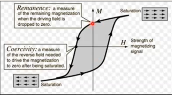
Example
A steel ring, with a coil around it. The ring is 0.2m long with area 400mm, the coil has 300 turns:
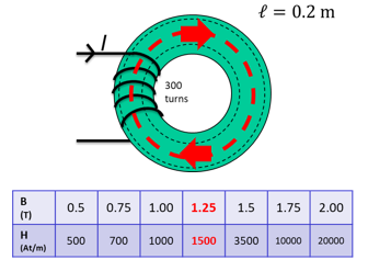
Calculate the magneto-motive force for 500 to flow, and the amount of current required to sustain this.
Flux density:
The field intensity is given from the table describing the hysteresis characteristics, . Relating magneto-motive force, current and field intensity:
Lenz's Law
The direction of an induced EMF is always such that the current it produces acts to oppose the change in flux or motion causing the induced EMF.
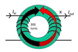
- A clockwise field is generated by the first coil
- The flux generated by the first coil links with the second coil's turns
- If this flux is changing, an EMF is induced in the second coil
- More turns = more linkage = more emf
- The EMF induces a current in the second coil
- The current in the coil causes it to generate it's own flux, in opposition to the flux of the first coil
- EMF out and current out are a function of the ratio between coil turns due to flux linkage
- This is how transformers work
To induce an EMF, the flux linking the coil must be changing, so typically an AC signal is used. The magnitude of this induced EMF is the rate of change of flux linkage
Reluctance and Force
An armature exposed to a magnetic field will try to move to the point in the field where the least resistance to flux exists
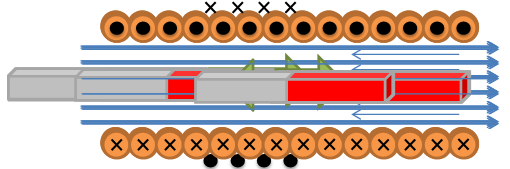
- A current is applied to a the coil to develop a field
- A soft iron bar is inserted which becomes magnetised
- The forced drags the bar in toward the centre of the coil
- As the bar moves in the field a counter current is generated in the coil due to Lenz's law, which reduces net field and force
- The field is not uniform, and is strongest in the centre
- The bar moves back and forth and eventually comes to rest in the centre of the field, where the force is strongest and reluctance is lowest
The energy stored in the coil does work by moving the bar, and the energy comes from inductance, the property of a magnetic field that defines its ability to store energy. THe voltage accross an inductor is given as:
Thus the power is:
The total work done in Joules is the integral of the power over time:
The force developed in a field is the Maxwell pulling force, and can be determined in several ways:
- is inductance in henries (H)
- is current in amps (A)
- is field length/air gap in meters (m)
- is coil turns
- is reluctance
- is material or air gap permeability
- is field area in square meters (m)
- is flux density in Teslas (T)
The equation relating flux, current, turns and inductance is:
PMDC Motors
Permanent magnet DC motors are widely used in a variety of applications due to their simplicity of control. They consist of two main parts: a stator, and an armature. Stationary magnets are attached to the stator, and coils of wire are wound around the rotating armature:
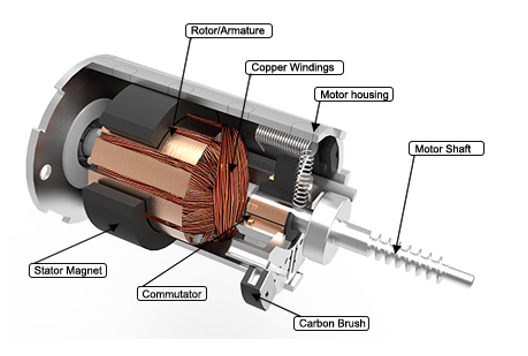
The circuit below is commonly used as a model of a PMDC motor:
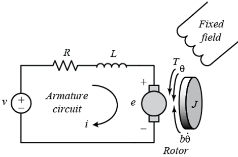
Using this model, the following equations can be derived:
- is applied voltage in Volts (V)
- is armature inductance in Henries (H)
- is armature resistance in ohms ()
- is inertia in kgm
- is friction in Nm/rad/s
- is the back emf constant in V/rad/s
- is the torque constant in Nm/A
- is torque load in Nm
- is current in Amps (A)
- is position in radians (rad)
Operating Points
The voltage applied causes motion, and the speed is determined by torque. The motor has linear relationsips in speed, torque, and current.
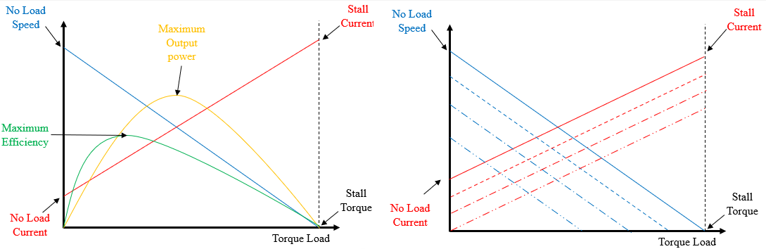
- For a given voltage, speed will decrease with torque and current will increase with increase torque
- The motor can operate over a range of input voltages
- The voltage applied determines the exact relationship between speed, current, and load
- If a certain known torque load wants to be driven at a certain speed, then a set input voltage can be calculated, which will draw a set amount of current
- To increase the speed of the same torque load, increase the voltage, which will increase the current
- The combination of speed, current, and load is the motor's operating point
Any given voltage and torque produces a speed and current, and the ideal operating point of a motor will be between the maximum efficiency and maximum output power points. When a motor is at a constant speed and current, the dynamic equations can be simplified to steady-state equations (also ):
Steady state current and velocity are therefore:
- Increasing will cause an increase in
- Increasing will cause a decrease in
- Increasing will cause an increase in
Power and Efficiency
The useful output power of a motor is rotational mechanical power. and are considered losses.
Input electrial power is , so electrical losses are mainly . The efficiency is output mechanical power over input electrical power:
Decreasing the friction will always increase efficiency, but as the other terms appear in both numerator and denominator, it is hard to find an optimum.
Wound DC Motors
Wound DC motors have a magnetic field generated by an electromagnet instead of a permanent magnet, so are generally more powerful and controllable.
- Separately excited DC motors use a source of current separate from the armature current to generate the field
- Series connected DC motors have the field windings in series with the armature
- Shunt connected DC motors have the field windings in parallel with the armature
Separately Excited
- Two separate input voltages
- Both windings used DC current
- Most controllable as field strength is isolated from armature current
- Mutual inductance couples the motor equations as the flux from and interact
- Used when a DC motor with high controllability and high power output is required, such as in electric trains
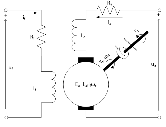
- , armature/field current
- , armature/field voltage
- , armature/field resistance
- , armature/field inductance
- mutual inductance
- armature inertia
- armature damping
- armature velocity
- torque load
Series Connected
- Self-exciting: no separate input to excite magnetic field
- Field lines are cut by armature field lines
- High starting torque
- Should not be run with no load as they have very high speeds
- Used in heavy industrial equipment with high torques
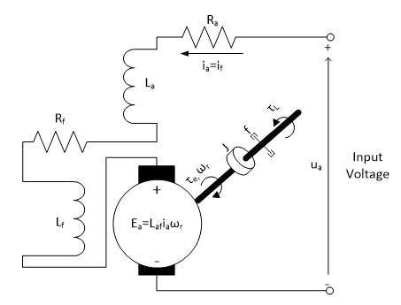
Shunt Connected
- Field windings are connected in parallel with armature windings
- Very good speed regulation
- Better at maintaining speed over a range of torque loads
- Best used where torque loads can vary ie in machining tools
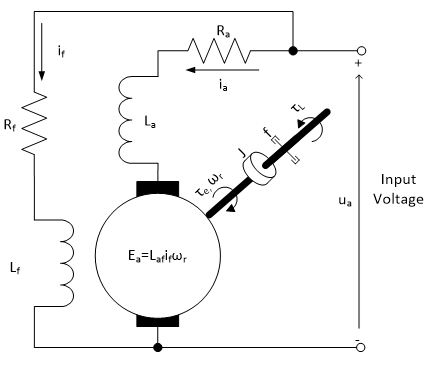
Motor Control
- Changes in speed are often required in a system.
- This can be done in PMDC motors by changing armature voltage
- Microcontrollers output a control signal to control the voltage
Pulse Width Modulation
- Works by providing a high-frequency square wave
- The ratio of high/low is called the duty ratio
- Effectively turns a transistor on/off very quickly
- Duty ratio determines voltage accross motor
The graph below shows a PWM signal along with the average voltages
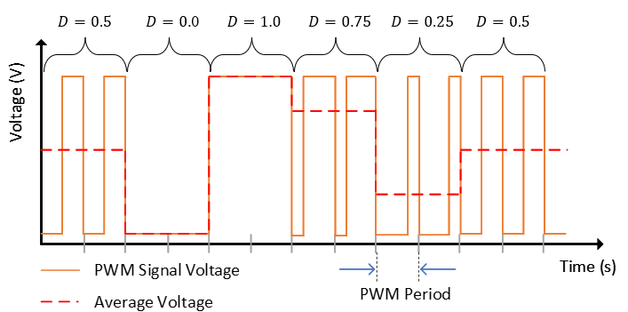
- The signal switches on and off very quickly, meaning the motor control circuit is turned on/off, but the motor has a high inductance meaning it does not respond as quickly
- This has the effect of averaging the voltage
- The PWM frequency is typically very high, and the period must be lower than the response time of the load
Motors can be modelled as an circuit with an inductance in series with a resistor, and an emf representing the motor's back emf:
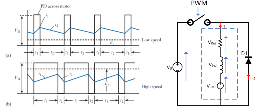
- The power supply is connected and disconnected by a switch controlled by PWM
- The instantaneous and average voltage accross the motor is shown on the graph for two different duty ratios
- The motor does not stop when disconnected because of the rise and fall time of the current in the RL circuit
- The diode is a freewheeling diode that allows a current path when the voltage switch is off
Low Side Drive Circuit
- The basic circuit for implementing motor speed control is shown below, known as a "Low Side PMDC Motor Drive Circuit"
- A high side version swaps the transistor and motor
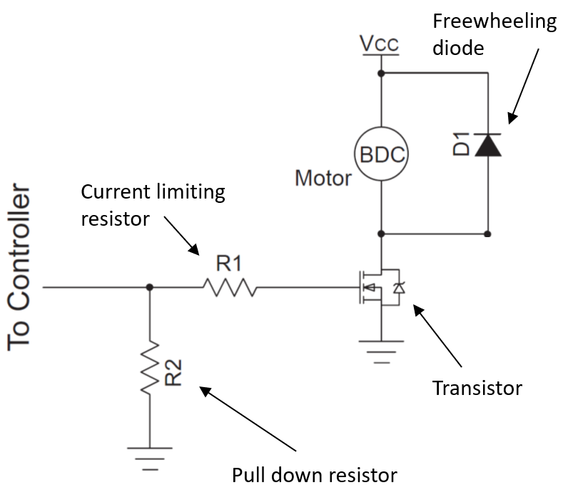
- The circuit is built around a transistor used to switch the voltage on and off
- N-type MOSFET generally the best choice
- Freewheeling diode provides a current path for motor current when the switch is off
- Typically a schottky diode
- Forward rated current should be greater than max current
- Reverse voltage should be higher than motor voltage
- Pull down resistor ensures transistor gate voltage is 0 when no input is applied
- Typically 10k
- Current limiting resistor protects transistor from damage
The signal from the controller will be connected to the transistor gate, switching on and off at the PWM frequency. The duty ratio determines the ratio of on/off, so the average voltage is:
H-Bridge
A H-Bridge is a power electronic circuit that can convert DC to AD current. For motor control, it can be used to drive a motor in either direction or apply PWM control.
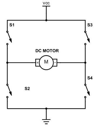
- The switches and , and and work in pairs
- The state of each pair should always be opposite
- Current flowing in different directions causes the motor to rotate in different directions
- There are also 3 other states:
- Shorting is when one side of the circuit has both switches closed and current flows straight to ground
- This is a short circuit and will cause damage
- Do not do this
- Braking
- and are closed, connecting both terminals to ground and causing the motor to brake sharply
- Coasting
- All switches open, motor will continue to spin until mechanical load brings it to a stop
- Shorting is when one side of the circuit has both switches closed and current flows straight to ground
Equations
Below are just the majority of the equations in one place without having to scroll :)
AC Power
The overwhelming majority of electrical power is AC power, single phase power from the mains at 240V 50-60 Hz.
Reactance of Capacitors and Inductors
When in parallel the impedances is:
RMS Power
AC voltages and currents alternate polarities so it is useful to define a DC equivalent, an average voltage/current. This is obtained by taking the root mean square of the sine wave:
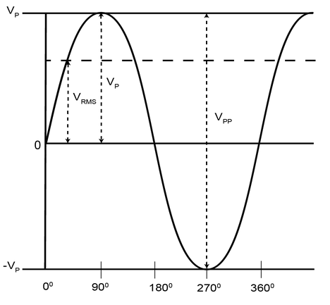
Real Power
Assume a simple circuit with just an AC source and resistor. The time taken for voltage and current to complete one cycle is . The power dissapated in a resistor over a full cycle is:
- There is a real power dissipated by a resistor
- Also called active, average or useful power.
- Measured in Watts
- Useful because it is converted to non-electrical forms like heat, light, or torque
Reactive Power
Assume a simple circuit with just an AC source and an inductor:
The power dissipated in one cycle is:
- The average power dissipated by an inductor is 0
- No useful work is done as there is no energy conversion
- Energy is exchanged between the magnetic field of the inductor and the power supply
- Instantaneous power is not zero
- Power consumed by a reactance is called reactive power and is measured in VARS (Volt-Amp Reactives)
- The same can be done for a capacitor, which exchanges energy between the power supply and it's electric field
Complex Power
- In a pure resistance, the voltage and current are in phase, and all power is positive and is dissipated
- In a pure reactance, the voltage and current are out of phase by 90 degrees, and the average power over a cycle is 0
- Instantaneous power, the power at any given point in time, is
- Most AC circuits contain both real and reactive components
- Resistors are real and dissipate active power in Watts
- Capacitors/inductors are reactive and dissipate reactive power in VARS
- The power supply will delive both real and reactive power in proportion to the magnitudes of real and reactive components
- Total power delivered is the complex power, a vector sum of real and reactive power
- Measured in Volt-Amps (VA)
Say an AC circuit applies a voltage accross an impedance , causing a current of to flow. The impedance can be written:
By Ohm's law:
is the load angle, which can be used to sketch a load triangle representing the complex power:
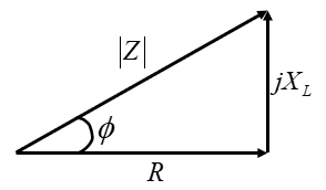
The load multiplied by the current square gives the power ():
is the complex power, comprised of the real and reactive power.
is the power factor. The closer it is to 1, the more real, useful, power is being dissapated in the system, which we want to maximise.
- If is positive, the power factor is lagging, meaning that the phase of the current is lagging the voltage
- The load is inductive, as current lags voltage in an inductance
- If is negative, the power factor is leading, current leads voltage
- The load is capacitive
Power Factor Correction
- Electrical power sources have to produce both real and reactive power
- Real power is useful and does work, reactive power does not
- Most reactive power is inductance in transmission lines
- We want to maximise the real power in the system, the ratio of which is given by the power factor
- Inductive loads cause a positive phase angle
- Lagging power factor as current lags voltage
- Capacitive loads cause a negative phase angle
- Leading power factor as current leads voltage
- Additional capacitors or inductors can be added to a power system to make the power factor as close to 1 as possible
The power triangle below shoes a reduction in reducing the reactive power but keeping the same real power
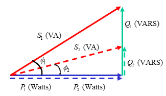
Example 1
Improve the power factor of the AC system shown to 0.98 lagging by adding a shunt reactance to the circuit
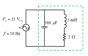
Reducing the system to a single impedance:
Calculating the complex power:
The current power triangle is therefore:
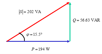
With a power factor of . The new load angle we require is . This will require a capacitance in parallel with the current impedance, which will dissipate more reactive power to give a new overall reactive power :
The shunt capacitance should have a value of to increase the power factor to 0.98 lagging.
Example 2
Add a component to this system to improve the power factor to 0.8 lagging.
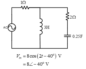
The total impedance of the system:
Calculating the power:
The current load angle is 14.6 lagging, so we need to add an inductance to make the system have a load angle of lagging
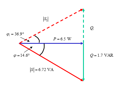
The power dissipated by the new inductor:
A shunt inductor of H is added to the system.
Resonant Circuits
- In any RLC circuit, it is possible to select a frequency at which the impedance is purely real
- At this frequency the circuit will draw only real power
- All the reactance will cancel out
- In cases where frequency is controllable this is useful to improve efficiency
- To calculate:
- Derive expression for the total circuit impedance
- Split into real and imaginary parts
- Derive a value of such that the imaginary part is 0
Example
Find an expression for the resonant frequency:
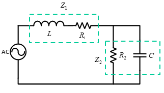
We require that such that :
Transformers
- Transformers are the link between power systems of different voltage levels
- Step-up and step-down voltage
- An increase in voltage gives decrease in current and vice versa
- Have full-load efficiencies of around 98% and are highly reliable
- Similar to how mechanical gears increase/decrease torque/velocity dependent upon gear ratio, electrical transformers increase/decrease voltage/current dependent upon turns ratio
- Consist of an iron/ferromagnetic core with wires wrapped around either side
![]()
- Changing voltage accross one coil induces magneto-motive force channelled through core
- The other coil links the changing flux, inducing a voltage accross it
Ideal Transformers
Ratios of input/output for an ideal transformer are given by:
When referring electrical properties over a transformer, multiply or divide by
An ideal transformer is assumed to be 100% efficient:
Example
A single phase, 2 winding transformer is rated at 20kVA, 480V/120V, 50Hz. A source connected to the 480V (primary) winding supplies an impedance load connected to the 120V (secondary) winding. The load absorbs 15kVA at 0.8pf lagging when the load voltage is 118V.
The turns ratio is given by the ratio of voltages:
The load accross the primary winding is then calculated based on the load on the secondary winding:
The current on the secondary side is calculated from the power:
The power factor is lagging so the current is lagging voltage, the current should have a negative phase angle:
The load impedance can then be calculated from this:
The load impedance referred over the transformer, as seen by the primary winding:
The real and reactive power supplied to the primary winding is calculated easily as this is an ideal transformer, so
Non-Ideal Transformers
In reality:
- Windings have resistance
- Core has a reluctance
- Flux is not entirely confined to the core
- There are real and reactive power losses so efficiency is not 100%
To model a transformer more accurately, introduce a resistance in series to model windings resistance, and inductance in series to model flux being not confined to core:
![]()
The model above shows a non-ideal transformer modelled with a single extra resistance and inductance, where the impedances from one side have been referred to the other to create a single impedance with values shown.
- Note that in large power transformers, the winding resistance is tiny compared to leakage reactance, so series resistances may sometimes be omitted.
Example
An example of a power system containing an ideal transformer is shown below. An AC generator with internal impedance ZGen is connected to a transmission line with impedance . The voltage is then stepped up by an ideal transformer with a turns ratio of 0.1 and supplies a load impedance of with a voltage . Find the real power dissipated by the line impedance and the voltage accross the load.
![]()
Refer the load accross the transformer to create a single circuit:
Now the circuit is a simple AC circuit with three impedences in parallel:
Current delivered by the generator:
Real power dissipated by the line impedance is:
To calculate the load voltage, we first need to refer current accross the transformer:
The load voltage is then:
Three Phase AC Systems
- 3 phase systems exist because generators are usually design to have 3 outputs
- Power is transmitted as 3 phase AC power
- The 3 phases are all AC signals 120° degrees out of phase with each other
- A balanced system has voltages and currents of the same amplitude and frequency shifted 120°
- Assumes all 3 transmission lines and loads have the same impedance
- Each of the three phases can be connected to identical loads, and the system would consist of three single phase circuits
- Phase sequence determines the order that the peaks of each phase pass
- Positive phase sequence means the peaks pass in the order ABC
- Phase A leads B by 120°
- Phase B leads C by 120°
- Negative phase sequence means the peaks pass in the order ACB
- Phase A leads C by 120°
- Phase C leads B by 120°
- Phasors are rotating clockwise
Star and Delta Connected Systems
There are two ways to connect 3 phase sources and loads:
- Star connected systems
- The negative of each phase is connected to ground
- Delta connected systems
- The negative of each phase is connected to another phase
- The phase voltage is the voltage between a phase and the ground, eg
- The line voltage is the voltage between two transmission lines, eg
- The phase current is the current flowing through a phase, eg
- The line current is the current flowing out of each phase, eg
Star Connected
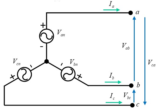
The phase voltages are measured accross a single phase:
- Line voltages are measured between each pair of lines, and are different from the phase voltages
- Phase currents are measure in each phase, and are the same as the line currents
Positive Sequence
All three line voltages are the phase voltages, and lead them by 30°:
All 6 voltage phasors are shown in the diagram below:
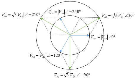
Negative Sequence
All three line voltages are the phase voltages, and lag them by 30°:
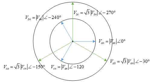
Delta connected
Phase voltages are measured accross a single phase:
- Line voltages are measured between the lines, and are the same as the phase voltages
- Phase currents are measured in each phase, and are different from the line currents
Positive Sequence
All three line currents are the phase currents, and lag them by 30°:
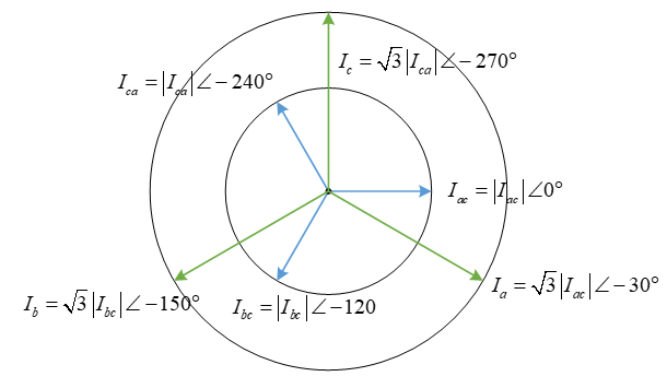
Negative Sequence
All three line currents are the phase currents, and lead them by 30°:
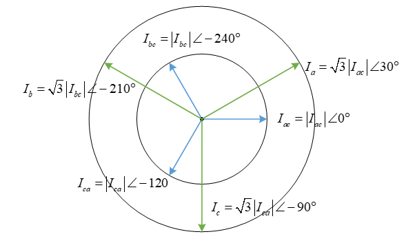
Three Phase Loads
- 3-phase loads can also be star or delta connected
- Phases are assumed to be balanced because shit gets fucked if they're not
- Sometimes it is necessary to convert between star and delta loads
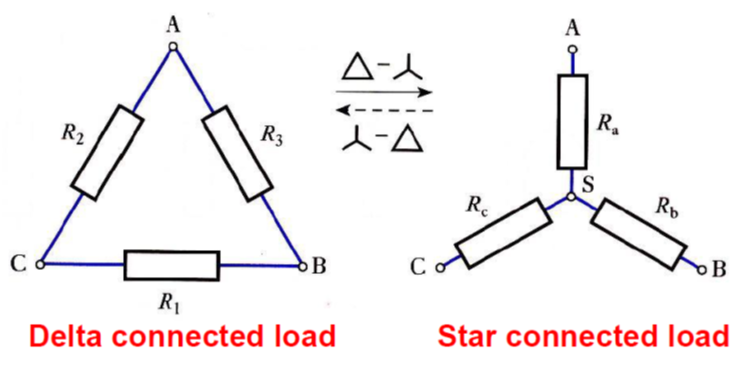
- denotes the load in a delta connected system
- denotes the load in a star connected system
Delta to Star
For a balanced load where :
Star to Delta
For a balanced load where :
System Configurations
There are four possible configurations of sources and loads. It easiest to perform analysis on star to star connected systems as it allows single phase analysis, so converting delta to star loads is often needed.
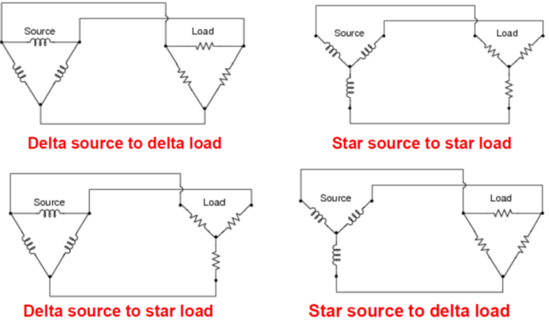
Power in Three Phase Circuits
The total power delivered by a 3-phase generator and absorbed by a three phase load is the sum of the power in each of the three phases, or 3 times the power in one phase in a balanced system. Power can be expressed in terms of phase voltages and currents.
For both star and delta connected loads:
| Power | Equation |
|---|---|
| Active power per phase | |
| Three phase active power | |
| Reactive power per phase | |
| Three phase reactive power | |
| Apparent power per phase | |
| Three phase apparent power |
Example 1
A balanced 3-phase star connected positive sequence source delivers power to a balanced 3-phase star connected load:
- Line-to-Line voltage at each source is
- Each transmission line had a resistance of 1 Ohm and an inductance of 9.5 mH
- Each phase is a 4 Ohm resistance and a 20 mH inductor
- System operates at 50Hz

Converting line voltage to phase voltage:
The impedance of the load and the transmission line :
The line and load current (they're the same in star systems) are calculated using the phase voltage and the total impedance:
The voltage across each phase load is the line current and the load impedance:
The total active and reactive power dissipated by all phases of the load can then be calculated:
The total active and reactive power consumed by the line:
Therefore the total complex power delivered by the source is:
Example 2
A balanced 3-phase star connected positive sequence voltage source delivers power to a balanced 3-phase delta connected load:
- Line-to-Line voltage at each source is
- Each transmission line had a resistance of 1 Ohm and an inductance of 9.5 mH
- Each phase is a 4 Ohm resistance and a 20 mH inductor
- System operates at 50Hz
The delta connected load must be converted to it's star equivalent, by dividing the impedences and phase shifting voltages and currents where necessary.
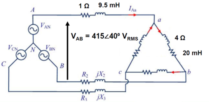
Converting line to phase voltage to get the voltage of each phase at the source:
The impedance of each line:
The impedance of each load, then converted to it's star equivalent to calculate individual line currents:
The line and phase currents in a delta load are different, so the line current is calculated from the source phase voltage and total impedance (star equivalent load and line impedances):
The phase current of the delta load can then be calculated from the line current:
The phase voltage of each delta load is then:
The power consumed by the load is then:
The power consumed by the line:
Total power delivered:
ES2C7
Binomial Theorem & Taylor Series
Binomial Theorem
Taking powers of binomial expressions yields binomial expressions, the coefficients of which form pascals triangle:
This can be generalised to:
For the particular case where and ,we have:
When is not a positive integer and :
Note that this is now an infinite series which converges. Can be used to approximate functions by ignoring higher order terms.
Sequences
A sequence is any arrangement of numbers, functions, terms, etc, in a specific order.
- May be finite or infinite
- The term of the sequence is denoted
A sequence of functions, :
Series
A series is obtained by summing a sequence
Arithmetic sequences/series have a common difference, , between terms
Geometric series are obtained by multiplying the previous term by a fixed number, the common ratio
Limits
It is important to know if a sequence converges to a value as , or diverges to as . Consider:
A sequence converges if it has a limit. If not, it diverges
Converge of Infinite Series
Manipulating the sequence can make it easier to see if the sequence converges or diverges. For example:
Divide by the highest power of k:
Since and both tend to 0 as , the sum is convergent.
Another example, consider the series
Clearly, , however the partial sum (the sum of terms up to ) has terms, the smallest being . Thus:
The series is divergent, as can be seen from the limit of partial sums. In order to see whether an infinite series converges to a limit, , (a finite sum for infinite number of terms) we look at the sequence of partial sums, , up to terms. Another example:
Sequence of partial sums:
The sequence of partial sums shows that the series converges.
- Infinite arithmetic series are always divergent.
- Infinite geometric series are convergent iff
- Sum is
Tests for Convergence
Comparison Test
A series of positive terms is convergent if the value of each of its terms is less than or equal to the corresponding terms of another series of positive terms that is convergent.
A series of positive terms is divergent if the value of each of its terms is greater than or equal to the corresponding terms of another series of positive terms that is divergent
Ratio Test
The series of positive terms
is convergent if:
and divergent if:
Example
Testing the following sequence for convergence:
Compare it with a sequence less than it that is known to be convergent:
Thus is convergent.
Taylor & Maclaurin Series
Taylor and Maclaurin series provide polynomial approximations to any function. Suppose that a function is infinitely differentiable, and its derivatives known at a particular point, . This function can then be expressed as an infinite polynomial series.
This series can be repeatedly differentiated to obtain values for all the constants:
Therefore the Taylor series expansion of about the point $x^{*} = a$ is:
Alternatively expressed as
Maclaurin Series
If expanding about the point , then the Taylor series becomes the Maclaurin series:
Example
Finding Maclaurin series for :
The image below shows the polynomial maclaurin approximations to for increasing . You can see how accuracy improves as
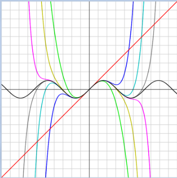
Matrices & Quadratic Forms
Linear Algebra
Linear algebra is the formalisation/generalisation of linear equations involving vectors and matrices. A linear algebraic equation looks like
where is a matrix, and , are vectors. In an equation like this, we're interested in the existence of and the number of solutions. Linear ODEs are also of interest, looking like
where is a matrix, is a vector, and is a function over a vector.
- I'm really not about to go into what a matrix or it's transpose is
- denotes the transpose of
- is a column vector, indexed
- is a row vector
- You can index matrices using the notation , which is the element in row and column , indexed from 1
Matrices can be partitioned into sub-matrices:
Column and row partitions give row/column vectors.
- A square matrix of order has dimensions x
- The leading diagonal is entries
- The trace of a square matrix is the sum of the leading diagonal
- A diagonal matrix has only entries on the leading diagonal
- The identity matrix is a diagonal matrix of ones
The Inner Product
The inner product of two vectors , a row vector, and , a column vector:
- (1x) matrix times (x1) to yield a scalar
- If the inner product is zero, then and are orthogonal
- In euclidian space, the inner product is the dot product
- The norm/magnitude/length of a vector is
- If norm is one, vector is unit vector
Linear Independence
Consider a set of vectors all of equal dimensions, . The vector is linearly dependent on the vectors if there exists non-zero scalars such that:
If no such scalars exist, the set of vectors are linearly independent.
Finding the linearly independent rows in a matrix:
- is independent of since for any
-
- Row 3 is linearly dependent on rows 1 and 2
- There are 2 linearly independent rows
- It can also be found that there are two linearly independent columns
Any matrix has the same number of linearly independent rows and linearly independent columns
A more formalised approach is to put the matrix into row echelon form, and then count the number of non-zero rows. in row echelon form may be obtained by gaussian elimination:
Minors, Cofactors, and Determinants
For an x matrix , the determinant is defined as
- denotes a chosen row along which to compute the sum
- is the cofactor of element
- is the minor of element
- The minor is obtained by calculating the determinant from the matrix obtained by deleting row and column
- The cofactor is the minor with the appropriate sign from the matrix of signs
Determinant Properties
- If a constant scalar times any row/column is added to any other row/column, the is unchanged
- If and are of the same order, then
- iff the rank of is less than its order, for a square matrix.
Rank
The rank of a matrix is the number of linearly independent columns/rows
Any non-zero x matrix has rank if at least one of it's -square minors is non-zero, while every -square minor is zero.
- -square denotes the order of the determinant used to calculate the minor
For example:
- The determinant is 0
- The rank is less than 3
- The minor .
- The order of this minor is 2
- Thus, the rank of is 2
There are two other ways to find the rank of a matrix, via gaussian elimination into row-echelon form, or by the definition of linear independence.
Inverses of Matrices
The inverse of a square matrix is defined:
- is unique
is the adjoint of , the transpose of the matrix of cofactors:
If , is singular and has no inverse.
Pseudo-inverse of a Non-Square Matrix
Given a more general x matrix , we want some inverse such that , or .
If (more columns than rows, matrix is fat), and , then the right pseudo-inverse is defined as:
If (more rows than columns, matrix is tall), and , then the left pseudo-inverse is defined as:
For example, the right pseudo inverse of :
Symmetric Matrices
A matrix is symmetric if
A matrix is skew-symmetric if
For any square matrix :
- is a symmetric matrix
- is a symmetric matrix
- is a skew-symmetric matrix
Every square matrix can be written as the sum of a symmetric matrix and skew-symmetric matrix :
Quadratic forms
Consider a polynomial with variables and constants of the form:
When expanded:
This is known as a quadratic form, and can be written:
where is an column vector, and is an symmetric matrix. In two variables:
Linear forms are also a thing. A general linear form in three variables , , :
This allows us to represent any quadratic function as a sum of:
For example:
Linear Simultaneous Equations
The general form of a set of linear simulatenous equations:
This can be rewritten in a matrix/vector form:
Equations of this form have three cases for their solutions:
- The system has no solution
- The system has a unique solution
- The system has an infinite number of solutions
- can take a number of values
An over-determined system has more equations than unknowns and has no solution:
An under-determined system has more unknowns than equations and has infinite solutions:
A consistent system has a unique solution
The solution for this system is . Note that the rank and order of are both 2, and exists in this case. If the determinant of a consistent system is 0, there will be no solutions.
Solutions of Equations
To determine which of the three cases a system is:
- Introduce the augmented matrix:
- Calculate the rank of and
No Solution
- If , then the system has no solution
- All vectors will result in an error vector
- A particular error vector will minimise the norm of the equation error
- The least square error solution,
Unique Solution
where is the number of variables in
- .
Infinite Solutions
- Paramaeters can be assigned to any elements of the vector and the remaining elements can be computed in terms of these parameters
- A particular vector will again minimise the square of the norm of the solution vector
Homogenous Systems
A system of homogenous equations take the form:
- is an x matrix of known coefficients
- is an x null column vector
- is an x vector of unknowns
The augmented matrix and , so there is at least one solution vector . There are two possible cases for other solutions:
- and , then the trivial solution is the only unique solution
- If and , then there is an infinite number of non-trivial solutions
- This includes the trivial solution
Example 1
Solutions to:
First calculate the determinant of :
so is a full rank matrix (rank = order = 3). We know solutions exist, but need to find the rank of to check if unique or infinite solutions. Using gaussian elimination to put into row-echelon form:
The rank of , so there is a unique solution
Example 2
Solutions to:
There is the trivial solution , but we need to known if there is infinite solutions, which we can determine from . Putting it into row-echelon form:
, so there is infinite solutions. Can introduce a parameter to express solutions in terms of. Using the coefficients from the row-echelon form:
Eigenvalues & Eigenvectors
For a square matrix , a scalar is an eigenvalue of , where:
This can be rewritten as a homogenous equation in an unknown vector :
This equation has infinitely many non-trivial solutions for , where:
This is the characteristic equation of , and the eigenvalues are scalars that satisfy this. Since the characteristic equation is an -th degree polynomial, an matrix will have eigenvalues for .
Corresponding to each eigenvalue , eigenvectors are non-trivial solutions of:
Example
Eigenvalues and vectors of:
The characteristic equation and it's solutions:
Eigenvector for :
Eigenvector for :
Spectral Decomposition
An x matrix has eigenvectors and associated eigenvectors .
is an x matrix of column eigenvectors, and is an x diagonal matrix of eigenvalues
for all matrices
In general, eigenvectors of are linearly independent and so exists. The spectral decomposition of a matrix can then be written:
This allows for diagonalisation of a matrix in terms of its eigenvectors, and for breaking down a multi-dimensional problem into a set of single dimensional problems.
- This is only possible if all eigenvectors are linearly independent.
- If any are repeated then this is not the case
If is a symmetric matrix, then the eigenvectors are mutually orthogonal, ie for all . If these eigenvectors are orthonormalised (of unit length), then the matrix of eigenvectors is an orthogal matrix, meaning its transpose is equal to it's inverse. Hence, the spectral resolution of a symmetric matrix is:
Example
Find the spectral resolution of, and hence diagonalise:
The eigenvalues of are and . These can then be used to compute the corresponding eigenvectors:
Using :
The spectral resolution of is given by:
can then be diagonalised by :
Oscillators & State Space Systems
Modal Analysis
Oscillators are coupled mass/spring, pendulums, etc systems, which can be analysed using modal analysis:
- Start with a complex coupled system
- Use spectral decomposition to diagonalise the system into simpler uncoupled systems
- Solve for each system
Single Degree of Freedom Oscillators
Mass-Spring
The equation of motion is:
where is the normalised stiffness, . Assuming an oscillatory solution:
Solving for by substituting back in gives .
Setting and :
This system oscillates at a single frequency, .
Pendulum
The equation of motion for a pendulum in the tangential direction is:
Where
- The system oscillates at the frequency
- This system has the same form, and therefore solution, as the mass-spring.
- The frequency depends only on the length, not the mass, a property unique to pendulums.
Multiple Degrees of Freedom
This single degree of freedom can be generalised to a 2nd order -degree of freedom system:
- is an matrix
- is an -dimensional column vector
The goal is to find frequencies such that the solution can be expressed as harmonic functions of . This is done by spectral decomposition:
Introduce a new variable , so that for :
This equation involving a diagonal matrix can then be decomposed to uncoupled scalar equations (the normal modes) for each scalar in :
This is a single degree of freedom scalar equation, as the previous two examples, thus:
The solution of the 2nd order -DoF system is defined by a superposition of the normal modes
- is an eigenvalue of
- is the frequency of the normal mode
- is an eigenvector of
- Specifies the shape of the normal mode
Example 1
Conside a system of two coupled masses:
- Two masses and
- Two displacements
- The variable to solve for
- Three springs , ,
Two equations of motion, one for each mass:
Rearranging into a matrix equation:
Let , and :
To solve the system, need to compute the eigenvalues and eigenvectors of , and hence the normal modes. Starting with the eigenvalues:
Hence the two natural frequencies of oscillation are and . Now for the eigenvectors:
The first mode , , implies that both bodies move in unison at the frequency of the mode $f = \frac{1}{\sqrt{2\pi}$Hz. The spring between the two masses does not stretch or contract.
The second mode , , implies that both bodies move in opposition at the frequency of the mode Hz, with the connecting spring stretching and contracting.
Example 2
The full nonlinear equations of motion for a double pendulum are:
Assuming small angles, and therefore neglecting square terms and making small angle trigonometric approximations:
Let:
To put into the form , we can premultiply by the inverse of the first matrix:
Now we have , we can compute it's normal modes.
Mode 1 :
- rad/s
- The system oscillates at a low frequency
-
- System oscillates in-phase
Mode 2 :
- rad/s
- The system oscillates at a high frequency
-
- System oscillates out of phase
The oscillation of the overall system will be the superposition of these two modes.
State Space Linear Systems
Consider a second order linear ODE of the form . Two variables are needed to uniquely specify the state of the system at any moment in time, the displacement , and the velocity . The system can be rewritten in terms of these:
This has replaced a 2nd order scalar equation with a two-state 1st order matrix equation. This concept can be generalised to express an th order linear ODE as an -state first order linear matrix ODE:
Where the state vector
Now to work out how to solve it. In the scalar case, the solution to with has the form
The sign of determines the stability of the system:
- is negative: the system decays exponentially and is stable
- is zero: nothing ever happens
- is positive: the system rises exponentially and is unstable
The matrix case has the same solution:
The task is then to compute the matrix exponential, and characterise the dynamics of the solution using the matrix .
Suppose has the spectral decomposition :
Defining again:
Since is diagonal, this is now a set of uncoupled equations:
are the individual modes of the solution and are defined by the eigenvalues alone. The matrix exponential is given by:
Multiplying by the starting state gives:
- The solution is a linear combination of the terms
- Hence, behaviour is defined by the eigenvalues
- The system is stable if all eigenvalues are negative
- If at least one is positive, the system is unstable
Example
Consider an elementary RLC circuit with all components in series, with a non-zero initial charge on the capacitor. The instantaneous charge in the circuit is described by a linear state space differential equation where and . Suppose:
Find the particular solution for this system and discuss it's stability.
The state space equation for the system in the form is:
The eigenvalues and eigenvectors of are:
The spectral resolution of :
The solution is given by , and the matrix exponential term :
Thus the solution:
Also, since both eigenvalues , the system is stable.
Differential Matrix Calculus
The Derivative of a Matrix
Consider where and is a scalar. The derivative of with respect to time is:
The derivative of a matrix with respect to a scalar is just the derivative of all the values. Similarly for an matrix
Vector-Valued Functions
The set of functions on the same variables can be represented as a vector-valued function over the vector
Each element of the vector is a function of the variables
- is an vector function over
- is an vector
The Matrix Form of the Chain Rule
If and such that :
This is the same as the scalar case, but note that matrix multiplication is not commutative so the order matters.
The Jacobian Matrix
The derivative of a vector function with respect to a column vector is defined formally as the Jacobian matrix:
The Jacobian matrix is the derivative of a multivariate function, representing the best linear approximation to a differentiable function near a point. Geometrically, it defines a tangent plane to the function at the point
Linearisation of a Matrix Differential Equation
Assume that is a stationary point (equilibrium state) of a non-linear system described by a matrix differential equation:
The linearisation of this system is the evaluation of the Jacobian matrix at . The linearised equation is , with the matrix of constants .
Example
Linearise the system around an equilibrium state:
, , and are parameters. At it's equilibrium,
There are three solutions to this system of algebraic equations, but we're interested in the one at the origin where . Evaluating the Jacobian at this point:
The linearised equation is therefore:
The Derivative of a Scalar Function With Respect to a Vector
If is a scalar quantity that depends on a vector of variables, then the derivative of with respect to $\mathbf$ is a row vector:
This is the gradient or nabla ()
The Derivative of the Quadratic Form
Using an auxillary result
We can compute the derivative of a quadratic form :
Since is symmetric by definition of the quadratic form, , the derivative of the quadratic form is a row vector:
Example
Consider the polynomial . Find . First putting the equation into quadratic form:
The derivative :
Optimisation
Multidimensional Taylor Series
The scalar case of the taylor series is an expansion of the function about the point :
This can be generalised to a matrix case. Let be a scalar function of a column vector . The taylor series expansion of about the point is:
This result is a scalar. Consider the first three terms:
is a row vector with it's gradient evaluated at the point :
is the matrix of second derivatives, called the Hessian matrix, evaluated at point
- The Hessian matrix is generally symmetric
- Matrix of mixed partial derivatives
Taylor series can be used to approximate multidimensional functions:
- Let be a scalar function of an vector ,
- Expand about a point , assuming displacements about
- The first term is a linear form
- Second term a quadratic form
- Higher order terms are ignored
Multidimensional Optimisation
Optimisation tasks involve finding such that is at an extremum (max/min).
Consider a continuous function , expanded about the point , with a vector as the displacement from :
The point is an extremum if the gradient vector when . The homogenous nonlinear equation therefore defines an extremum .
If , then:
Therefore:
This is the important result that defines the extremum of a function
To determine the nature of the extremum, the sign of the must be determined. By the spectral resolution, this is determined by the eigenvalues of . It is said that the sign definiteness of is determined by
Let be a quadratic form m, where is a symmetric matrix. The eigenvalues of are . The definiteness is determined by all of the eigenvalues:
| Definiteness of | Nature of Point | |
|---|---|---|
| Positive Definite | Minimum | |
| Positive Semidefinite | Probable Valley | |
| and | Indefinite | Saddle Point |
| Negative Semidefinite | Probable Ridge | |
| Negative Definite | Maximum |
Extrema of a Multivariate Quadratic
For a quadratic , the extremum is at the point where :
A maximum/minimum exists at the point if the matrix is positive/negative definite.
Example 1
Find the extremum (and it's nature) of the quadratic function:
Put into matrix form:
The extremum of this quadratic form exists at the point where:
To determine the nature, find the eigenvalues of :
The eigenvalues lie either side of zero, which makes indefinite, and the extremum is therefore a saddle point.
Example 2
Find the stationary points (and their nature) for the function:
The stationary points lie where :
The solutions are therefore:
Two solutions:
To determine the nature of the extremum, we need the hessian matrix:
The eigenvalues at each point will give the nature. For :
The hessian matrix is positive semidefinite, so the point is probably a valley, but further analysis is required to determine the nature of the point.
For :
The hessian matrix is indefinite, so the point is a saddle point.
Fourier Series and Transforms
Fourier Series
Fourier series provide a way of representing any periodic function as a sum of trigonometric functions. For a periodic function with period , the Fourier series is given by:
Where the coefficients and are called the Fourier coefficients, integrals calculated over the period of the function:
Note that if the function is even , then the term is always 0, and the series is comprised of cosine terms only:
Likewise for odd functions , the term is always zero, and the series is comprised of sine terms only:
The Fourier series uniquely represents a function if:
- The integral of function over its period is finite
- The function has a finite number of discontinuities over any finite interval
- Most (if not all) functions/signals of any engineering interest will satisfy these conditions
Exponential Representation
The Fourier series can be rewritten using Euler's formula :
Note that T = 2L, the period of the function.
Frequency Spectrum Representation
The spectrum representation gives the magnitude and phase of the harmonic components defined by the frequencies contained in a signal
This gives two spectra:
- The frequency spectrum, describing the magnitude for each frequency present in the signal
- The phase spectrum, describing the phase for each frequency present in the signal
The diagram below shows the frequency spectrum for the functions and , respectively:
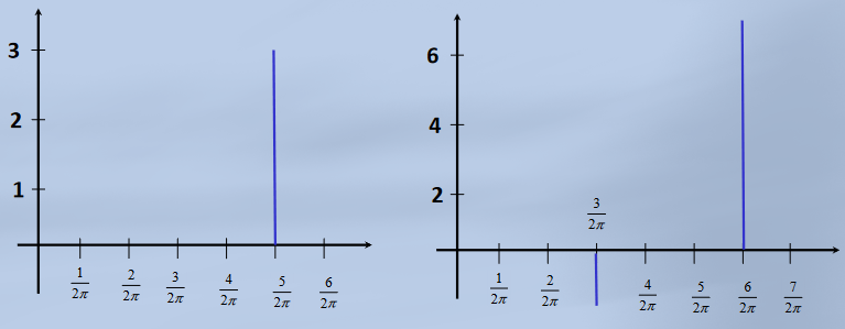
Example
Find the fourier series of the following function:
is an odd function with period (), hence we only need the integral:
Since :
Can introduce a new index , such that :
The Fourier series for is therefore given by:
Fourier Transforms
Fourier series give a representation of periodic signals, but non periodic signals can not be analysed in the same way. The Fourier transform works by replacing a sum of discrete sinusoids with a continuous integral of sinusoids over frequency, transforming from the time domain to the frequency domain. A non-periodic function can be expressed as:
Provided that:
- and are piecewise continuous in every finite interval
- exists
This can also be expressed in complex notation:
- is the Fourier transform of , denoted
- is the inverse Fourier transform of , denoted
For periodic signals:
- Fourier series break a signal down into components with discrete frequencies
- Amplitude and phase of components can be calculated from coefficients
- Plots of amplitude and phase against frequency give frequency spectrum of a signal
- The spectrum is discrete for periodic signals
For non-periodic signals:
- Fourier Transforms represent a signal as a continuous integral over a range of frequencies
- The frequency spectrum of the signal is continuous rather than discrete
- gives the spectrum amplitude
- gives the spectrum phase
Fourier Transform Properties
Fourier transforms have linearity, same as z and Laplace.
Time Shift
For any constant :
If the original function is shifted in time by a constant amount, this does not affect the magnitude of its frequency spectrum . Since the complex exponential always has a magnitude of 1, the time delay alters the phase of but not its magnitude.
Frequency Shift
For any constant :
Example
Find the Fourier integral representation of
This is the Fourier transform of . Using Euler's relation :
Therefore, the integral representation is:
Z Transforms
Difference Equations
A difference equation is a discrete equivalent of a differential equation, used in situations where only discrete values can be measured:
becomes
These can be solved numerically by just evaluating the output for each value of n. For example:
This evaluates to:
Alternatively, there is an analytical solution...
The z Transform
Consider a discrete sequence . The z transform of this sequence is defined as:
A closed-form expression can generally be found by the sum of the infinite series. For example, the z transform of the unit step :
This is a geometric series with , , hence the sum is
Taking a z transform of a difference equation converts it to a continuous function. The z domain is similar to the laplace domain, but for discrete time signals instead.
Common z Transforms

z Transform Properties
z transforms have linearity, the same as laplace and fourier transforms.
First Shift Theorem
If is a sequence and it's transform, then
For example, if :
For :
Second Shift Theorem
The function is defined:
Where is the unit step function. The function , where is a positive integer, represents a shift to the right of this function by sample intervals. If this shifted function is sampled, we have . The second shift theorem states:
Inverse z Transforms
z transforms are inverted using lookup tables, but to get them into a recognisable form, some manipulation is often needed, including partial fractions. For example, finding the inverse transform of :
The first term can be seen immediately from the table:
The second term rearranges to give:
This is in the form of the second shift theorem, so this can be applied to give:
Thus,
Example
Solve , where , .
Taking z transforms:
Rearranging and using initial conditions:
Using partial fractions:
Using inverse transforms straight from the table to get the solution:
Partial Differential Equations
PDEs are use to model many kinds of problems. Their solutions give evolution of a function as a function of time and space. Boundary conditions involving time and space are used as initial conditions.
A method of separation of variables is used for solving them, where it is assumed that . Two other auxiliary ODE results are also needed:
Another auxillary ODE are needed for some situations
The general process for solving PDEs:
- Apply separation of variables
- Make an appropriate choice of constant
- Nearly always
- Solve resulting ODEs
- Combine ODE solutions to form general PDE solution
- Apply boundary conditions to obtain particular PDE solution
- Work out values for the arbitrary constants
Laplace's Equation
Laplace's equation described many problems involving flow in a plane:
Find the solution with the following boundary conditions:
- and
- as
Starting with separation of variables:
Substituting back into the original PDE:
We have transformed the PDE into an ODE, where each side is a function of / only. The only circumstances under which the two sides can be equal for all values of and is if both sides independent and equal to a constant. Since the constant is arbitrary, let it be . Now we have two ODEs and their solutions from the auxiliary results earlier:
Substituting the solutions back into , we have a general solution to our PDE in terms of 4 arbitrary constants:
We can now apply boundary conditions:
- Substituting in gives
- Substituting in gives
- Using the two together gives , so either:
- If , then , so
- This is the trivial solution and is of no interest
- If , then
- This also implies that , so is useless too
The issue is that we selected our arbitrary constant badly. If we use instead, then our solutions are the other way round:
Checking the boundary conditions again:
- First condition,
- Gives
- Second condition
- Gives
- Either (not interested)
- is an integer,
- Gives
We now have:
Where is any integer. Using the other boundary conditions:
- as
- If is positive, then (otherwise )
- If is negative, then (otherwise )
Taking as positive, the form of the solutions is:
The most general form is the sum of these:
Applying the final boundary condition:
- for all other
The complete solution is therefore:
The Heat Equation
The heat equation describe diffusion of energy or matter. With a diffusion coefficient :
Solving with the following boundary conditions:
Separating variables, , and substituting, exactly the same as Laplace's equation, we have:
Setting both sides again equal to a constant , we have two ODEs (one 2nd order, one 1st):
The general solution is therefore:
Tidying up a bit, let , , :
Applying the first boundary condition:
- Gives
- Since for all ,
We now have . The second boundary condition:
- , so
- For the non trivial solution ,and since ,
- Therefore, for
Substituting this in gives:
The above equation is valid for any , so summing these gives the most general solution:
The last boundary condition is :
This is in the form of the a Fourier series:
We have:
Substituting this into , and letting :
The Wave Equation
The wave equation is used to describe vibrational problems:
Solving the equation with the boundary conditions:
Doing the usual separation of variables and substitution, and choosing a constant :
Solving both ODEs:
This is the general solution. Start applying boundary conditions:
- implies that
- As this is true for all ,
- implies that
- This is also true for all , so
- Required that , so
- for
We now have:
Applying the third boundary condition, :
As this is for all , , so . We now have:
The general solution is then:
Applying the final boundary condition of , gives , else . The particular solution is therefore:
ES2E3
Flash cards:
The ever so kind Aaron has made some flashcards. They are somewhat brief and don't cover everything, but they are better than nothing :)
Click here for quizlet.
Logic
Whilst its only recapped on in some of the lectures, it assumes knowledge from the engineering module, which the computer science Computer Organisation and Architecture (CS132) also covers.
A fair bit of this information is already in CS132 Logic Page. There are some engineering specific things, and stuff that's just handy to have on one page.
Boolean Algebra Laws
There are several laws of boolean algebra which can be used to simplify logic expressions:
| Name | AND form | OR form |
|---|---|---|
| Identity Law | ||
| Null Law | ||
| Idempotent Law | ||
| Inverse Law | ||
| Commutative Law | ||
| Associative Law | ||
| Distributive Law | ||
| Absorption Law | ||
| De Morgan's Law |
- Can go from AND to OR form (and vice versa) by swapping AND for OR, and 0 for 1
Most are fairly intuitive, but some less so. The important ones to remember are:
Latches
SR Latch
- When is asserted, goes high.
- When is asserted, goes low.
- When both are de-asserted (low and low), holds its value
- When both are asserted (high and high), and goes low (not intended!)
D latch
Passes through the input whenever is high, and hold when is low.
D Flip Flop
Will copy the input to the output at rising edges of . Bit storage.
Hardware Description Languages
So far, we've been restricted to describing circuits using equations and diagrams. Diagrams can convey structure, but behaviour can be hard to see and they become unweildy as they grow. HDLs are languages that describe hardware with a heirarchical design.
History
- Programmaple Array Logic (PAL) allows for implementing a sum of products logic, building circuits by blowing fuses in certain places.
- This got cumbersome for larger circuits
- PALASM developed as a language for mapping functional specifications to PAL
- Other languages developed around this concept, all with the idea of introducing more layers of abstraction
- There are two main languages in use today:
- Verilog
- VHDL
- Verilog started as a proprietary language, released to the public in 1991 and standardised in 1995 by the IEEE
- Standard revised in 2001
- SystemVerilog is an extension of Verilog with more capabilities
Verilog
- Verilog designs are broken down into modules
- A module is an encapsulation of a unit of functionality
- Good designs have appropriate levels of hierarchy
- At each level, modules below are treated as black boxes
- Modules are declared using the
modulekeyword and a list of ports- Can indicate the direction of the port as
inputoroutput endmoduleindicate the end of a module
- Can indicate the direction of the port as
- Identifiers are the names of modules, signals, ports, etc
- Must start with a letter, and can't clash with keywords
- Wires can be declared within modules using the
wirekeyword - Verilog is case sensitive, ignores whitespace and uses C-style
//comments
Structural Verilog Design
- Circuits are described structurally, by the structure of their constituent parts
- Primitives are included for all basic gates:
and(x, a, b)is equivalent toor(z, a, b, c, d)is equivalent to- Arguments are either ports or wires declared within module
Consider an and-or inverter:
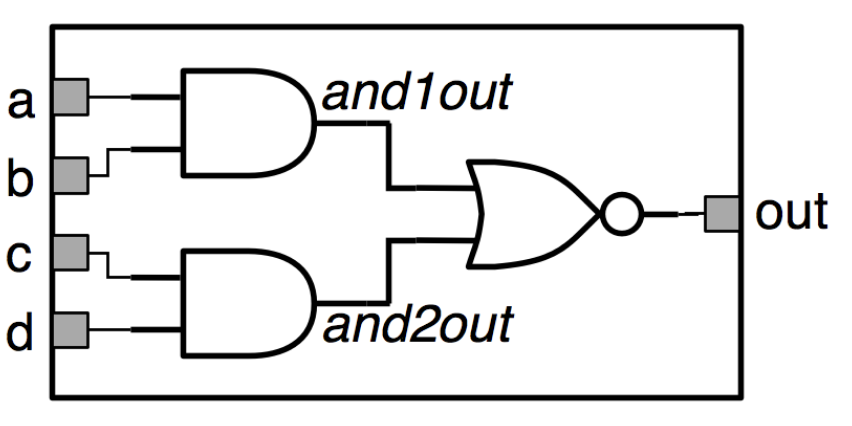
module andorinv (input a, b, c, d, output out);
wire and1out, and2out;
and (and1out, a, b);
and (and2out, c, d);
nor(out, and1out, and2out);
endmodule
Note the two internal wires being used here. Gates can also be given identifiers, which helps with testing and readability:
module andorinv (input a, b, c, d, output out);
wire and1out, and2out;
and g1(and1out, a, b);
and g2(and2out, c, d);
nor g3(out, and1out, and2out);
endmodule
The order of statements in Verilog is irrelevant, as each statement describes a piece of hardware, so there is no sequence of steps, unlike when writing procedural code.
It is also important to obey the usual connection rules for combinational circuits:
- Every node of the circuit is either an input, or connects to exactly one output terminal of a gate
- The same wire cannot be driven by multiple gates
- There can be no cycles in the circuit
Structural Verilog
- Have seen how to write Verilog for combinational modules consisting of gates
- Each time we use a gate, we are creating an instance of that gate connected to the wires in the brackets
- This concept extends to all Verilog modules
Binary Adder
A half adder takes two 1-bit inputs and generates a sum and a carry out:
| A | B | sum | carry |
|---|---|---|---|
| 0 | 0 | 0 | 0 |
| 0 | 1 | 1 | 0 |
| 1 | 0 | 1 | 0 |
| 1 | 1 | 0 | 1 |
Can see there are two gates in this design:
- Sum is an XOR
- Carry is an AND
Can express in verilog as follows:
module add_half(input a, b //two inputs two outputs
output sum, carry);
xor g1(sum,a,b); //xor gate for sum output
and g2 (carry,a,b) //and gate for carry output
endmodule;
Full Adder
A full adder is similar but accepts a carry in to chain carries out
| Cin | A | B | Cout | Sum |
|---|---|---|---|---|
| 0 | 0 | 0 | 0 | 0 |
| 0 | 0 | 1 | 0 | 1 |
| 0 | 1 | 0 | 0 | 1 |
| 0 | 1 | 1 | 1 | 0 |
| 1 | 0 | 0 | 0 | 1 |
| 1 | 0 | 1 | 1 | 0 |
| 1 | 1 | 0 | 1 | 0 |
| 1 | 1 | 1 | 1 | 1 |
Can see that this is made using half adders:
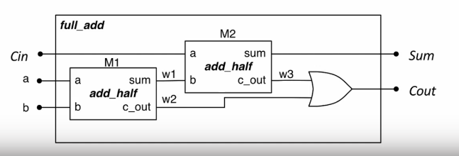
Structural verilog allows for building modules from other modules to create a hierarchy. Can instantiate our half adder module twice to reuse it in our full adder module to create a hierarchical design.
module full_add(input a, b, Cin,
output sum, Cout);
wire w1, w2, w3;
//instance of add_half
add_half m1 (a, b, w1, w2);
add_half m2 (Cin,w1,sum,w3);
or(Cout,w2,w3);
endmodule;
Instantiation in Verilog
- Instantiate a module by invoking its name and then naming that instance
- Example above creates two
add_halfs namedm1andm2 - Connects the signals and ports referenced in the parentheses with the corresponding ports of the instantiated module
- Same as gate modules
- Order of signals determines connections
- This is error prone, as it requires to remember the order of the ports
- If port specification is changed, have to change the instantiation
- Should always instead use a named connection:
add_half(.a(a), .b(b), .sum(w1), .Cout(w2))
The port name for the module is preceded with a dot ., and the internal port is given in brackets.
Assign Statements
Verilog has assign statements to express combinational logic
assign result = a & b;
This is called a continuous assignment: it allows us to assign the result of a boolean expression to a signal. there is a range of bitwise operators:
| Operator | Function |
|---|---|
& | AND |
| | OR |
~ | NOT |
^ | XOR |
~& | NAND |
~| | NOR |
Here is the full adder from earlier using assign statements instead of gates. There is no need to describe the structure in terms of gates, only logic functions. As with gate instances, the order of assign statements is irrelevant.
module full_add(input a, b, Cin,
output sum, Cout);
assign sum = a ^ b ^ Cin;
assign Cout = (a & b) | (b & Cin) | (a & Cin);
endmodule;
It is also possible to assign implicitly in a wire declaration:
wire y;
assign y = (a & b) ^ c;
// equivalent to
wire y = (a & b) ^ c;
User-Defined Primitives
Verilog also allows you to create your own primitive modules which are defined using a truth table (though this isn't used much).
- Can only have one output and it must be the first port
?signifies a don't-care condition
primitive mux_prim(output mux_out,
input select, a, b);
table
// select a b : mux_out
0 0 ? : 0;
0 1 ? : 1;
1 ? 0 : 0
1 ? 1 : 1
? 0 0 : 0
? 1 1 : 1;
endtable
endprimitive;
Conditional Assignment
It is possible to have conditional assignment. Output is assigned to one of two possible expressions, dependant upon a condition:
// a multiplexer
assign y = sel ? x1 : x0;
The signal y will be connected to x1 if sel is 1, else it will be connected to x0.
Multi-bit Signals
Verilog supports multi-bit signals, called vectors or buses. A signal is declared as a bus by specifying a range:
wire [31:0] databus; //32-bit bus
//ports can also be multiple bits wide
module add16(input [15:0] a, b,
output [15:0] sum,
output cout);
By convention, ranges are specified [MSB:LSB], meaning a 16-bit signal is [15:0]. The range is specified preceding the signal name.
Numeric Literals
Literals use the format <size>'<radix><value>
- size is the width of the number in bits
- radix is
binarydecimal,octal orhexadecimal 4'b0000- 4 binary bits 0000
8'h4F- 8 bit wide hex number 4F
8'b0100_1111- 8 bit wide binary number
- Underscores can split long strings
1'b1- A single
1bit
- A single
Working with Vectors
When using the vector name, all the bits are being operated on. Logic operations performed on vectors are bitwise.
wire [3:0] a = 4'b0110;
wire [3:0] b = 4'b1010;
wire [3:0] x = a & b;
wire [3:0] y = a ^ b;
Can access parts of a vector by specifying a range after the signal name
assign y = some[3];- Assign 4th bit of signal
someto y
- Assign 4th bit of signal
- `assign z = some[4:3];
- Creates two bit signal z from 5th/4th bit of
some
- Creates two bit signal z from 5th/4th bit of
The widths of vectors in assignments should match. Verilog doesn't check and will let you do:
assign x[2:0] = y[1];
assign x[2:1] = a;
This is probably not what you wanted to do. Always check widths and remember that LSB is 0.
Combinational Arithmetic
Verilog supports basic arithmetic and comparison:
- Arithmetic
+,-,*,/ - Comparison
- Return
1for true and0for false
- Return
assign sum = a+b;
assign diff = curr - prev;
assign max = (a > b) ? a : b;
Vectors are all treated as unsigned numbers
Parameters
Constants that are local to a module that can be optionally redefined on an instance-by-instance basis.
module some_mod#(parameter SIZE=8)
(input[SIZE-1:0] X, Y
output[SIZE-1:0 Z])
When module is instantiated parameters can be changed. The module above is instantiated twice below, but each instance is 16 bits:
module some_other_mod(input [15:0] a, b, c, output [15:0] D, E);
some_mod #(.SIZE(16)) U1 (.X(a), .Y(b), .Z(D));
some_mod #(.SIZE(16)) U1 (.X(c), .Y(b), .Z(E));
endmodule;
Concatenation and Replication
Signals can be concatenated into a single signal using brace syntax.
//b is 8 bit
assign b = {a[3:0], 4'b0000}
wire [3:0] a, b;
wire [7:0] y;
//join two 4 bit signals to create 8 bit bus
assign y = {a,b};
Signals can also be replicated with a preceding integer or variable.
//c is also 8 bit
assign c = {4{a[3]}, a[3:0]};
Example: 2-bit comparator
A verilog module to compare two 2-bit signals a [1:0] and b [1:0]
module comp_2bit (input [1:0] a,b output a_gt_b);
assign a_gt_b = //complex combinatorial logic
//alternatively
assign a_gt_b = (a > b);
endmodule;
Behavioural Verilog
- Rather than describe how the circuit is constructed or it's raw function, describe how it behaves
- Implementation tools work out how to make hardware that fulfils the behaviour, considering the target architecture
The always block
An always block contains procedural statements that describe the behaviour of the required hardware.
always @ (a,b)
begin
x = a & b;
y = a | b;
end
- The
alwayskeyword starts a block - The sensitivity list (in brackets after the
@) contains the names of any signals that affect the block's output- The block is sensitive to
aandb - Signals the circuit should respond to
- Shorthand
always @ *includes all signals in sensitivity list
- The block is sensitive to
- Procedural statements between
beginandend - Give a more readable description of logic by describing how the output should change.
assignkeyword not used - always block is an alternative to using it
reg signals
- Since we are modelling at a higher level of abstraction, we use something other than wires
- Signals assigned to from within
alwaysblocks must be declared as of typereg - A
regis like a wire but can only be assigned to from within an always block- A wire is a connection between components and does not have its own value
- Cannot assign to a reg using an assign statement or use it to connect to the output of a module
- If you want to assign to an output port from inside an always block, it must be declared as
regin the module header too
The following two are functionally equivalent:
// x and y must be reg
always@ *
begin
x = a & b
y = a | b
end
//and
assign x = a & b;
assign y = a | b;
if Statements
Allows to describe a combinational circuit at a higher level of abstraction
always @ *
begin
if (x < 6)
alarm = 1'b0;
else
alarm = 1'b1
end
end
- Each branch can have more than one statement
- Use begin and end the same as braces in C
- Statements can be nested with other
- Condition can be anything the evaluates to a boolean value
- Can use comparisons and equality operators
- Can combine conditions with logical operators
!,&&,||
case Statements
Verilog features case statements that let us choose from multiple possibilities, similar to C.
always @ *
case (sel)
2'b00 : y = a;
2'b01 : y = b;
2'b10 : y = c;
default: y = 4'b1010;
endcase
A decoder is a good use case for a case statement
module decoder3_8(input [2:0] ival, output reg [7:0] d_out);
always @ *
case(ival)
3'b000 : d_out = 8'b00000001;
3'b001 : d_out = 8'b00000010;
//etc...
3'b111 : d_out = 8'b10000000;
endcase
endmodule
Can also describe a multiplexer:
module mux4 (input [3:0] d, input [1:0] sel, output reg q)
always @ * begin
case (sel)
2'b00 : q = d[0]
2'b01 : q = d[1]
2'b10 : q = d[2]
2'b11 : q = d[3]
endcase
end
endmodule
- Can assign to multiple signals from inside one always block
- If you assign to a signal from inside an always block, must never do so anywhere else
- Using
assign - In another always block
- Like connecting a wire to multiple inputs: not allowed
- Using
- Order matters in an always block as we are describing behaviour
- If a signal is assigned to more than once, the last one takes precedence
Avoiding latches
always @ *
begin
if (valid) begin
x = a | b;
y = c;
end
else
x = a;
end
- What happens to
yin the else branch? No output is specified - No output is explicitly specified
ylatches on previous value- Not ideal
- All outputs from the always block must be assigned to in all circumstances
- An output not being assigned to implies it should be latched or stored
- If no output is specified, output is no longer combinational
- Compiler would understand it to be a latch
A way to avoid this is to always use a default assignment at the top of the always block. The default will be overwritten by any subsequent assignments
always @ * begin
y = x;
if(valid) begin
c = a | b;
y = z;
end
else
c = a;
// y is x here
end
end
- Must always include any signal that is in the sensitivity list
- Must assign to an output signal in all possible cases
- This is to maintain combinational logic
FPGA Design Flow
How do you go from HDL to a circuit? The key development was tools that could take HDL and generate a circuit automatically. Design flow is the process by which we specify and design a system all the way through to implementation.
The Design Process
- Design is always informed by a specification
- What does the circuit do?
- What I/O does it need?
- Performance requirements
- Space/Power budget
- Edge cases
- This is the most important stage as it defines what the design will be verified against
- Also influences the choice of target architecture
- Errors in interpretation of the specification/requirements can cause issues
- Next is design entry
- Writing the actual HDL files
- Modules and sub-modules are defined
- I/O is defined
- There are two main aspects to architecture design
- The datapath, logic that acts on data to compute the required functions
- The control path, logic that manages the movement of data and controls the datapath
- Functional verification is performed throughout the design process
- It is important to verify that the HDL meets the specification
- Usually start at the lowest level modules and move up
- This is an iterative process, and testing should be continuous
- Synthesis is the process by which the design is converted into circuits
- Lots of optimisation goes on at this stage
- Combinational logic is minimised
- Arithmetic operators are expanded into primitive operations
- Basic structures like memories, multiplexers, decoders are inferred
- The result of synthesis is a netlist, a low-level representation of the circuit using basic blocks
- Mapping takes the netlist and works out how to build it on the target architecture
- For ASIC design, each node in the netlist is mapped to cells from a cell library
- For FPGA design, each node is mapped to resources available on the FPGA
- Maps combinational logic to LUTs
- Synchronouse components mapped to flip-flops
- Arithmetic mapped to ALUs or DSPs
- This gives an architecture-specific netlist
- Synthesis verification checks the circuit is valid
- Checks circuit fits on FPGA
- Estimates timing, power usage, performance
- Place and Route is when the netlist is mapped onto specific locations on the FPGA, and routing is configured to connect the blocks
- Often multiple iterations are needed to get it right
- Timing verification checks timing constraints have been met
- The bitstream is a file that is loaded onto the FPGA that tells it how to configure itself
Intellectual Property
- IP cores are premade designs
- Implementing complex hardware is pointless when you can re-use other modules
- Similar to software libraries
- Lots of open source cores are available online
- Vendors and FPGA companies sell IPs
- Good IP works as a black-box
- Well-defined
- Configurable
- Thoroughly tested and verified
- Provided with data sheets like any other piece of hardware
FPGA Architecture
Anything written in HDL will probably eventually end up as a real circuit that the mapping tool has to generate from basic components.
- In ASICs, CMOS is the most common technology, however:
- Fabrication is complex and expensive
- Designs are inflexible
- High-start up costs
- FPGAs are more attractive because they are cheaper and more flexible
- ASICs can be cheaper for large volumes however, so there is a cost tradeoff
Understanding FPGA architecture gives us a better understanding of the mapping process to make our circuits easier to map, and to make most efficient use of FPGA resources. There are primarily four distinct types of resources on an FPGA:
- Flexible logic: basic configurable blocks to implement combinational logic, coupled with clocked elements to enable synchronous logic and pipelining
- Flexible routing: signigicant chip area dedicated to wires and switch boxes that enable connections between all components
- Flexible I/O: multi-standard interfacing to external pins, with a range of speed capabilities
- Embedded hard modules: an number of different resources optimised for speed and area, including DSPs and memories
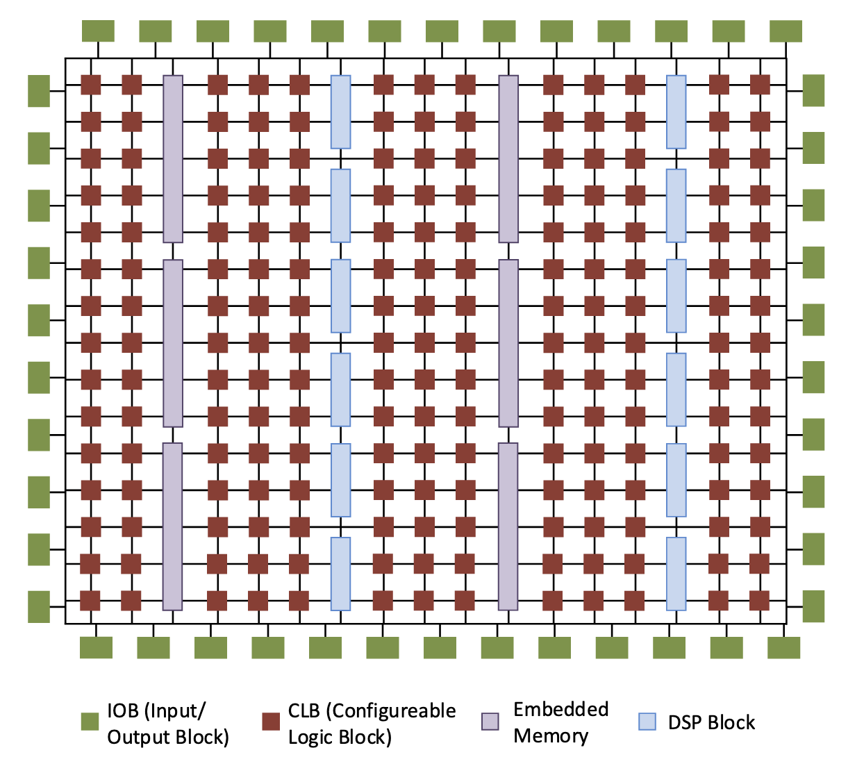
Logic Blocks
- Logic blocks do most of the computation on FPGAs
- Made up of basic elements called Configurable Logic Blocks (CLBs), which consist of:
- A LUT to implement combinational functions
- Some arithmetic logic
- Flip-flops
- LUTs and flip-flops can be used together or independently
- Most FPGAs are built using SRAM technology
- An n-input LUT is just a x 1-bit memory
- The truth table for the function is stored in the LUT
- When an input pattern is applied, the bit at the corresponding location is the output
- The propagation delay through a LUT is independent of the function it computes
- LUTs can be broken down for smaller functions or combined for larger functions
- LUTs are grouped together in groups of 4 to form a slice
- Slices also contain clocked elements, ALUs, etc
- Multiple slices form CLBs
- LUTs can also be used as mini-memories to form distributed RAM
- Each 6-input LUT can also implement a 32-bit shift register, without using the flip-flops in the slice
Routing
- There is a large grid of wires throughout the FPGA
- Connection boxes allow different elements to connect to this network
- Switch boxes allow tracks to connect to each other
- Place & route tools work out how to most efficiently make these connections
- Routing is a key factor in the performance of a design
- Longer wires = higher latency
- Dedicated wires between blocks exist and are faster and save the general routing for other uses
- The individual bits of multi-bit wide signals may take different routes
- As architectures evolve, connectivity keeps improving
- A mix of wire lengths helps improve performance
I/O
A key feature of FPGAs is highly flexible I/O.
- Individual groups of pins can be interfaced according to different standards
- High end FPGAs include high-speed serial interfaces
- Support for 10GigE, SATA, PCIe
- IP blocks included to configure these
- On modern FPGAs, rates of over 32 Gb/s can be achieved
Block Memory
LUTs can implement very small memories, but hard blocks of synchronous memories are also included as block RAMs.
- 36Kb, and can be split into two 18Kb blocks
- Can run at well over 500MHz
- Support different sizes and configurations
- All the features of a high-end memory system
DSP
FPGAs excel in Digital Signal Processing applications, so modern FPGAs include hard DSP blocks.
- Usable for any multiply/add/accumulate operations
- Highly parallel dataflow arrangement
- Much faster than LUTs
DSP blocks are highly configurable
- Configurable number of pipeline stages
- Dynamically configurable ALU function
- Dynamically configurable bypass for pre-adder and multiplier
- Can cascade signals for combining DSP blocks
Synthesis and mapping tools work out how best to utilise all the resources most efficiently, but Verilog should always be written to optimise for and take advantage of the target architecture.
Sequential Verilog
- We can design combinational circuits using
- Gate-level structural design
- Assign statements
- Behavioural always blocks
- Important to consider that our circuits are purely combinational in all cases
- It is possible to design sequential circuits
- Most designs will be synchronous: synced with a clock
Latches
SR Latch
- Two inputs
- Two outputs
- Two NOR gates
module srlatch(input R, S
output Q, Qbar);
nor N1 (Q, R, Qbar);
nor N2 (Qbar, S, Q);
// Alternatively
assign Q = R ~| Qbar;
assign Qbar = S ~| Q;
endmodule
D Latch
A D latch is synchronous, where an SR isn't:
module dlatch(input EN, D,
output reg Q, Qbar);
always @ (D, EN)
if(EN) begin
Q <= D;
Qbar <= ~D;
end
end
endmodule;
D goes to Q if enable is high: circuit is described succinctly.
Generally, FPGA designs will be synchronous as it allows us to more easily understand the timing of the circuit. Most of the logic we will look at will be edge-triggered, which is described as follows:
module simplereg(input d, clk, output reg q);
always @ (posedge clk)
q <= d;
endmodule
posedge keyword can can be used in a sensitivity list to define a trigger on the rising edge of a clock (negedge is also a thing). In this case, a simple register is created. A multi-bit register/flip flop is defined below:
module simplereg(input [3:0] d, input clk, output reg [3:0] q);
always @ (posedge clk)
q <= d;
endmodule
Clocks and Reset
- All circuits should be synchronised based on the same clock signal
- Clock can be named whatever (usually
clk) and defined as an input to the module - We often need to reset the contents of a register or state of circuit to 0/a default
- Two types of reset:
- Asynchronous: whenever the reset input is asserted, the reset is triggered
- Synchronous: if the reset is asserted on the rising edge, reset is triggered
- In modern FPGA design, we use synchronous reset
- Two types of reset:
An 8 bit register with synchronous reset:
module 8bitreg(input [7:0] d,
input clk, rst,
output reg [7:0] q);
always @ (posedge clk) begin
if(rst)
q <= 8'b00000000;
else
q <= d;
end
endmodule
For an asynchronous reset, the reset signal is added to the sensitivity list so that the block can be triggered independently of the clock. However, this will desynchronise the always block from the rest of the circuit so is not the prefferred way to do it.
module 8bitreg(input [7:0] d,
input clk, rst,
output reg [7:0] q);
always @ (posedge clk or posedge rst) begin
if(rst)
q <= 8'b00000000;
else
q <= d;
end
endmodule
Registers
Can control multiple registers from the same block. Each assignment in a synchronous always block creates a register controlled by the same block. This verilog module contains 3 8-bit registers.
module multireg(input [7:0] a, b, c
input clk, rst
output reg [7:0] q, r, s);
always @ (posedge clk) begin
if(!rst) begin
q <= 0;
r <= 0;
s <= 0;
end
else begin
q <= a;
r <= b;
s <= c;
end
end
endmodule
- When drawing can ignore clock and reset as they should always be there
- Putting a triangle on an input in a block diagram shows that the input is edge-triggered
Non-Blocking assignment
- The
<=operator is called non-blocking assignment - For combinational always blocks, as use blocking assignment and order matters
- For a synchronous block, order does not matter
- Everything only happens on the rising edge
Counters
A register where the value increments on the rising edge (or decrements if down signal is asserted).
module simplecount(input clk, rst, down, output reg [3:0] q);
always @ (posedge clk) begin
if(rst)
q <= 4'b0000;
else
if(down)
q <= q - 1'b1;
else
q <= q + 1'b1;
endmodule
Can alter to include an enable signal. Since it's a synchronous component, don't need to account for all branches.
module simplecount(input clk, rst, down, enable, output reg [3:0] q);
always @ (posedge clk) begin
if(rst)
q <= 4'b0000;
else
if(enable)
if(down)
q <= q - 1'b1;
else
q <= q + 1'b1;
end
endmodule
Can again alter to include the ability to load a value.
module simplecount(input clk, rst, down, load, input [3:0] cnt_in, output reg [3:0] q);
always @ (posedge clk) begin
if(rst)
q <= 4'b0000;
else
if(load)
q <= cnt_in
else
if(down)
q <= q - 1'b1;
else
q <= q + 1'b1;
end
endmodule
Shift Registers
1 bit serial in serial out shift register. Propagation occurs on the rising edge of the clock.
- Order of assignment does not matter
module shiftreg(input clk, y, output reg q);
req q1,q2,q3;
always @ (posedge clk) begin
q1 <= y;
q2 <= q1;
q3 <= q2;
q <= q3;
end
endmodule
Can make the module simpler using vectors, where each stage in the shift register is a separate position in the vector. The LSB is replaced by the input, and the MSB is the output.
module shiftreg(input clk, y, output reg q_out);
req [4:0] q;
always @ (posedge clk) begin
q[0] <= y;
q[4:1] <= q[3:0];
q_out <= q[4];
end
endmodule
Memory
- 64 element memory requires 6-bit address input, with each word as 16 bits
- Declare internal 64-element array, where each position is 16 bits.
module spram(input clk, en, write_en,
input [5:0] addr,
input [15:0] d_in
output reg [15:0] d_out);
reg [15:0] ram [0:63];
always @ (posedge clk) begin
if (en) begin
if (write_en) begin
ram[addr] <= d_in;
end
d_out <= ram [addr];
end
end
endmodule
On each clock cycle:
- output 16 bit word that is on the provided addres
- if
write_en, thend_inis stored at the memory locationaddr
Finite State Machines
Take a binary counter as an example, the output of which is a sequence of numbers, increasing by one each step. The behaviour is described in terms of a register and an incrementer circuit. This is fairly easy to reason about as a state machine:
- At each point in time the system is in a state that determines what the output is (the contents of the register)
- On each transition, the state changes (counter increments)
This is a state machine. A finite state machine describes a system using a finite number of states, and associated transitions. In synchronous design, an FSM is in one state for the duration of each clock cycle, and may transition on each rising edge depending upon the input.
State transition diagrams show the different states of a system and transitions between them. The diagram below shows a 3-bit binary counter with an enable signal. The state only transitions if enable is high.
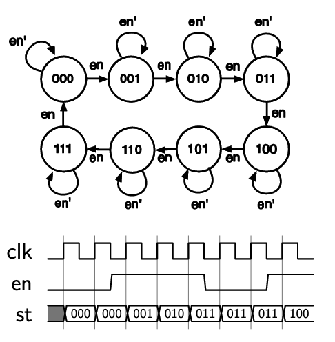
The diagram consisits of nodes with states, edges between the states, and conditions that determine which transitions may occur. Diagrams may be simplified by only including conditions that result in state-changing transitions:
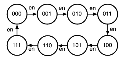
Consider an up/down counter:
- Two input signals,
dnanden - Counts up when
enis high - Counts up when
dnis low, down whendnis high - An input of 10 is
enhigh anddnlow- Other combinations with
en= 0 result in no transition
- Other combinations with
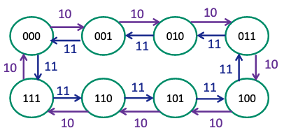
States can be labelled with a more meaningful name, like in the example below
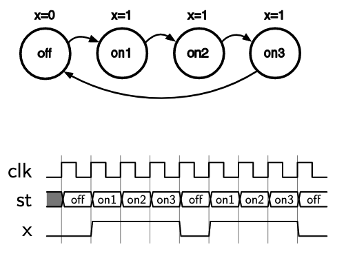
This FSM always produces 3 high cycles followed by one low, with the output x shown with the states. The FSM is off in the off state, and then on for the three on states.
The diagram below shows the same FSM, but it will only output the three-cycle pulse when an input signal b is set high. The output of each state is also shown in the circle next to the state: state/output. It is important to label diagrams with a proper legend to make it clear what means what.
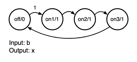
State transition information can also be presented in tables, which is effectively a truth table for the next state based on the current state
| Current state | Input b | Next state | Output x |
|---|---|---|---|
| off | 0 | off | 0 |
| off | 1 | on1 | 0 |
| on1 | 0 | on2 | 1 |
| on1 | 1 | on2 | 1 |
| on2 | 0 | on3 | 1 |
| on2 | 1 | on3 | 1 |
| on3 | 0 | off | 1 |
| on3 | 1 | off | 1 |
Can see that the state only transitions from off to on1 when input b is asserted.
Implementing FSM
Using a state table, you can build the combinational circuit that determines the next state from the current state. Connected with a register holding state, this forms the structure of a finite state machine.
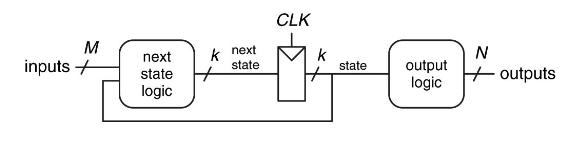
Consider an example of designing a lock that only unlocks (output u = 1) when input buttons are pressed in a fixed sequence. Inputs are 4 buttons: start, red, blue, green, and an input that indicates if any button has been pressed.
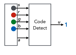
We can capture the lock's behaviour in a state diagram:
- Start in an initial state
- If start is pressed then move to another state (input
s) - If a button is pressed and its red, move to next state (input
ar)- So on for button presses
- If at any point a button is pressed but it is not the correct one, go back to the start again
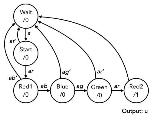
However their is still another issue, where if someone holds down all the buttons the machine will just cycle through to the end state. This can be fixed by attaching conditions to check that other buttons aren't pressed to the states, ensuring the machine is robust with regards to the requirements.
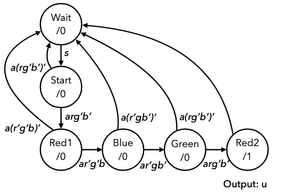
Consider another example of a vending machine:
- Accepts only £1 and 50p coins
- Dispenses drink for £1.50 and change if necessary
- Two inputs, c100 for £1 coin, c50 for 50p coin
- Assume only ever 1 input high, and it tells us which coin is inserted
- Two outputs, vend to release a drink, and change to give 50p of change.
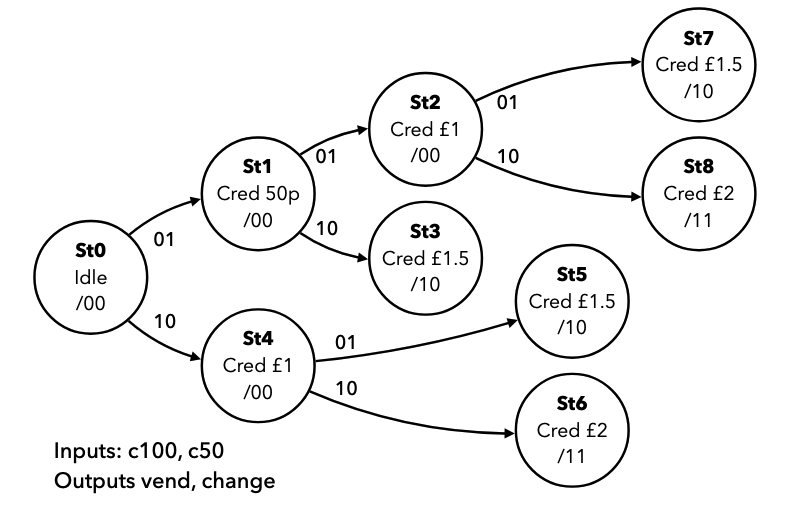
However, notice that some of these states are equivalent. These can be merged to reduce the number of states in the diagram, hence simplifying it
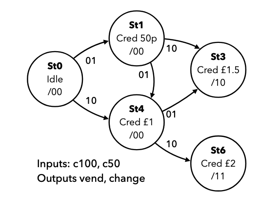
Moore and Mealy Machines
In all the previous examples, outputs depend only on the state. These are called Moore Machines. The alternative is Mealy Machines, where the output depends on the state and the current value of the inputs. Mealy machines are harder to design and analyze, but can be more compact. In mealy machines, the outputs cant be drawn in the state circles, so are added to the edges, as output is a function of state and input. The diagram below shows a previous example with the outputs on the arrows.
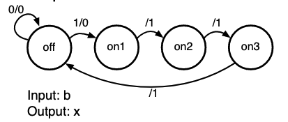
The two diagrams below show the same machine, that outputs a 1 when the last two inputs were 0 then 1.
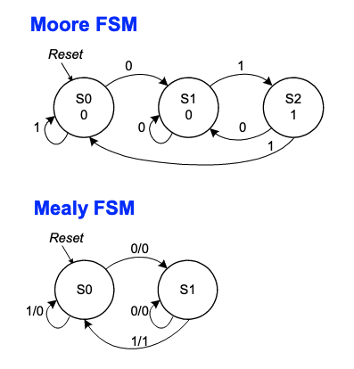
State Encoding & Transition Logic
In a synchronous design, we can assume that the FSM changes states only on rising edges, so we can put together a circuit like this, with a register and two sets of combinational logic:
- The state register stores the current state
- To encode state, a binary value is assigned to each state
- Need bits for states
- Must also build the transition logic
- This can be done from a state table, by replacing names with encodings
Consider the state transition logic for the example with the three-cycle pulse:
Current state: s[1:0] | Input b | Next state: ns[1:0] | Output x |
|---|---|---|---|
| 00 | 0 | 00 | 0 |
| 00 | 1 | 01 | 0 |
| 01 | 0 | 10 | 1 |
| 01 | 1 | 10 | 1 |
| 10 | 0 | 11 | 1 |
| 10 | 1 | 11 | 1 |
| 11 | 0 | 00 | 1 |
| 11 | 1 | 00 | 1 |
This is now a binary truth table, from which we can determine equations for each output bit, mapping s to ns.
ns[1] = s[1] & !s[0] | !s[1] & s[0]ns[0] = !s[1] & !s[0] & b | s[1] & !s[0]x = s[1] | s[0]
We can now create the two circuits and connect them into a state register. As a Verilog module, this requires a register, an always block, and combinational assignments connecting s and ns.
module pulse3 (input clk, rst, b, output x);
reg [1:0] s;
wire [1:0] ns;
assign ns[1] = s[1] ^ s[0];
assign ns[0] = (!s[1] & !s[0] & b) | (s[1] & !s[0]);
assign x = s[1] | s[0];
always @ (posedge clk) begin
if (rst) begin
s <= 2'b00;
end else begin
s <= ns;
end
end
endmodule
When implementing a finite state machine, always ensure the state register as a reset, and a defined initial state, otherwise the starting state of the FSM is unpredictable.
More Complex FSM
More complex FSMs with more states and inputs can be hard to construct truth tables and equations for. Verilog's behavioural abstractions can be used instead.
- Each state can be assigned a binary value and used as a named constants
- Still need two registers for the state and next state
- Synchronous logic to move state into next state
- Behavioural combinatorial
alwaysblock with a case statement for state transitions
Consider the more complex example with the button lock again:
module lock(input clk, rst, s, r, g, b, a, output u);
//define states as parameters
parameter wt = 3'b000, str = 3'b001, rd1 = 3'b010,
blu = 3'b011, grn = 3'b100, rd2 = 3'b101;
//state registers
reg [2:0] nst, st;
//output logic
//output u is only high when state is rd2
assign u = (st == rd2);
//synchronous logic for changing state
always @ (posedge clk) begin
if (rst) st <= wt;
else st <= nst;
end
//input logic
//combinatorial logic for defining state transitions
always @ * begin
nst = st;
case(st)
wt:
if(s) nst = str;
str:
if(a)
if(r&~b&~g) nst = rd1;
else nst = wt;
rd1:
if(a)
if(b&~r&~g) nst = blu;
else nst = wt;
blu:
if(a)
if(g&~r&~b) nst = grn;
else nst = wt;
grn:
if(a)
if(r&~g&~b) nst = rd2;
else nst = wt;
rd2:
nst = wt;
default:
nst = wt;
endcase
end
endmodule
The general structure of a state machine will always follow the example above.
- Always ensure next state is assigned in every case
- Use a default next state and output assignment at the top of the state transition block to minimise the number of statements
- Using a combinatorial
alwayblock, it becomes easy to verify that the FSM is correct, as we can verify against the state transition diagram.
Verification
Testbenches
Testing by loading to the FPGA takes ages. Testbenches allow for easier verifying correctness of verilog designs.
- Algorithmic verification: is the selected algorithm suitable for the desired application?
- Functional verification: does the designed architecture correctly implement the algorithm?
- Synthesis verification: is the design fully synthesisable and implementable on the target design platform?
- Timing verification: once synthesised, placed, and routed, does it meet timing constraints?
Sources of error in design
- The specification may be incorrect or incomplete
- Even if it meets specification, it may not function as intended
- Specification may have been misunderstood
- What has been implemented matches what you think the specification means, not what it actually means
- Specification has been implemented incorrectly
- Errors in code
Most of our time will be spent in functional verification.
- Does design perform all functions in spec?
- Are all required features implemented?
- Does it handle corner/edge cases?
What is a testbench?
- A self contained module, with no inputs or outputs
- Instantiates the unit under test (UUT) - the module we want to verify
- Contains a number of blocks
- Clock generator for driving synchronous elements
- Data and control signal generators for mimicking circuit inputs
- Data and status signal monitors for checking outputs match spec
If the module under test gives correct results when given inputs, then we can assume that it works.
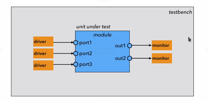
In verilog, a testbench is just a normal module with no ports:
module testbench;
//testbench statements
endmodule
The inputs to our unit under test will be driven by the testbench and must be declared as reg signals. Outputs must be declared wire. Inputs and outputs are then connected to the instanted module to be tested.
Initial Block
- Another type of procedural block used in testbenches only
- Cannot be synthesised
- Runs concurrently with always blocks
- Used to initialise values when system first starts up
- Can also set values with delay using
#10 a = 1'b1;statements- This tells the simulator to wait 10 time steps and then set a to 1
- Delays are only for simulation and cannot be synthesised
display
- The simulator has a console where the simulator prints messages
- The
displaytask/function allows us to print info to the console - Allows for C-style format strings
- Argument can be an expression also
Verifying Combinational Modules
We want to verify a simple combinational module that computes y = abc + a'bc' + ab'c'. Manually stimulate the inputs to cover all 8 possible input values:
module simplecomb(input a,b,c, output y);
assign y = abc + a'bc' + ab'c';
endmodule
module comb_test();
reg at,bt,ct;
wire yt;
simplecomb uut(.a(at),.b(bt),.c(ct));
initial begin
at = 1'b0;
bt = 1'b0;
ct = 1'b0;
//increment every 10 time steps
#10 ct = 1'b1;
#10 bt = 1'b1; ct = 1'b0;
#10 ct = 1'b1;
#10 at = 1'b1; bt = 1'b0; ct = 1'b0;
#10 ct = 1'b1;
#10 bt = 1'b1; ct = 1'b0;
#10 ct = 1'b1;
#10 \$finish;
end
endmodule
- Unit under test is instantiated, connecting ports to signals
- Start with input values for
a, b, cof 000 - Wait 10 timesteps and change inputs to
001 - Continue cycling through all possible values
\$finishterminates simulation- We want to see what output waveform is generated by the module so we can verify it exhibits the correct behaviour
Checking the waveform manually is tedious, so we can instead add assertions into testbench to \$display an error if the output does not match the expected value
at = 1'b0; bt = 1'b0; ct = 1'b0;
if(yt != 1'b0) \$display("000 failed")
//.. and so on
This is still tedious, as we still have to work out the correct value in advance. We could carry out the verification using verilog's language features instead:
always #10
if (yt != (a&b&c | (!a)&b&(!c) | a&(!b)&(!c)))
\$display("testbench failed for %b %b %b",a,b,c);
In testbench design we can be much more relaxed about using language constructs:
initialis not synthesisable but is fine in testbenches- Delays on assignments can be used
- Assigning to a signal from multiple blocks is not an issue
Testbenches are not designed to be turned into circuits: they are software, not hardware.
Synchronous Verification
- For synchronous testbenches, we need a clock input to oscillate between 0 and 1
- Initial value (high or low) is important and can be done either way
- Verilog below sets clock to change on each timestep (50% duty cycle)
initial clk = 0;
always #1 clk = ~clk;
Timing in Testbenches
- So far, we have assumed dimensionless time
- We can specify the time dimensions
timescale 1ns / 100ps- This line is placed at the top of the testbench source file
- Specifies unit time is
1ns - Specifies max rounding precision to be
100ps#10/8would give 1.2, not 1.25
- Most simulation tools require the timescale to be stated in order to simulate
- During functional simulation this means nothing since timing is not factored in
Since for most designs, clock and reset behaviour is the same, we can use a standard template:
module sync_test;
reg clk, rst;
initial begin
\$display("Start of Simulation");
clk = 1'b0;
rest = 1'b1;
#10 rest = 1'b0
end
always #5 clk = ~clk;
endmodule
Reset is held high for 10 time steps, then brought down to enable circuit. Clock oscillates continually.
Accessing files
- The set of inputs driving the circuit is a test vector
- Creating test vectors within a testbench is generally only feasible for simple parts of a circuit
- It is also possible to access test data stored in external files
- Allows us to prepare more complex types of test data, eg images
- Can also store simulation outputs in an external file
- Allows for analysis using more suitable tools, eg scripting with matlab/python
- File I/O in verilog is very similar to C
- Need a file handle (stored as an
integer) - Can use read/write/append mode
r/w/a
- Need a file handle (stored as an
- A self-checking testbench can be constructed by reading a set of inputs and outputs from files, and seeing if the unit under test matches them
integer infile;
infile = \$fopen("inputfile.txt","r");
while (!\$feof(infile)) begin
@(posedge clk);
\$fscanf(infile,"%h","%b\n",data,mode);
end
This example reads one hex and one binary value on each line of a test file in each clock cycle, and assigns them to the data and mode signals.
Advanced Verification
- When working with testbenches, should always use the same clock throughout
- If driving an input reg signal on one clock, that data will only enter the module at the next rising edge
- Simple combinational circuits can be tested using counters and inspection of outputs
- For more complex circuits, prepare test data and load from/write to files
\$randomfunction generates a 32-bit random number and can be used for random testing- If there are too many input possibilities, focus on edge cases or cases more likely to cause error
- Finite state machines are nicely decomposed for testing
- Test combinational state transition logic separately
- Test the whole state machine, manipulating inputs.
- Testing process should be iterative and integrated.
How to verify
- Start with a good design specification
- Prototyping is important: develop a prototype first
- Software models can be constructed of at various levels
- Simple model with no reflection of hardware design
- Model that mimics overall functional architecture
- A cycle-accurate model
- A bit-accurate model
- Mode detailed models give a better reflection of the hardware, but take longer to develop (and can have more bugs)
- A functionally correct circuit should produce the same results as a software model of the function, however some discrepancies may still be present
- Number representation can cause differences
- May use different calculation methods
- Can take shortcuts or refactor parts of an algorithm to simplify implementation in hardware
- Should be aware of these discrepancies and know when it is safe to ignore them
- Can apply the same set of input vectors to the hardware design and software model and compare the outputs
- Can also implement the inverse function in software
- Run data through hardware module
- Put outputs into software inverse
- If software inverse outputs original hardware inputs, design is correct
Simulation Environments
- Vivado comes with simulator built in
- Waveform window shows signals in design
- Signal values plotted as wave over time
- Useful for debugging
- More complex designs require more complex verification techniques
Modern Verification
- There have been many recent developments in electronic design automation around verification
- SystemVerilog adds new verification features
- Formal mathematical circuit verification involved proving a design is correct
- Sources of error can occur in places other than the design
- Faulty specification
- Buggy tools
Consider a large multiprocessor SoC:
- Test each processor and all layers in a hierarchy
- Test communication and interfaces
- Test contention for resources
- Test different clocks for different units
- Predict effects of cache misses and race conditions
For simple systems we work with:
- Prepare a software model
- Construct testbenches for simple logic
- Use self-checking testbenches if possible
- Use external files for test data if appropriate
- Make testing an iterative process
Testing can and should consume most of your time!
FPGA Arithmetic
FPGAs demonstrate their power specifically in applications that require complex computation at high data throughput, so the specifics of how arithmetic is carried out is important.
Number Format
- The binary number format is positional
- The value of a binary number is the sum of each element multiplied by it's position
- The rightmost bit is the LSB
- Leftmost bit is MSB
- Bits are indexed by their power
- LSB is bit 0
- MSB is bit n-1
- The range of an unsigned n-bit number is
- Sign-magnitude can be used to represent signed numbers
- An offset can also be used, where the number range is shifted by an amount
- Two's complement is mostly used where the MSB has a negative weight
- To negate a number, invert the bits and add 1
- If MSB = 1, the number is negative
- Has range to
- To widen a two's complement number, you need to sign extend
- Add more bits to the left with the same value as the current sign bit
Adders
The full adder allows to carry out a full add operation on two operands, producing a sum and carry ouput. This can be extended into a ripple adder, which is multiple adders chained together to create multi-bit adders.
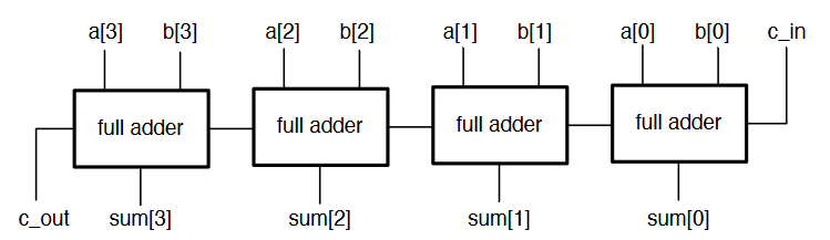
- Carry bits are passed up the chain from LSB to MSB
- The carry ripples through the circuit
- We have to wait for all the carry bits to propagate through the circuit to get the correct result
- Not efficient
The ripple adder can also be adapted to be able to subtract using XOR gates, and by adding one using the input carry bit.
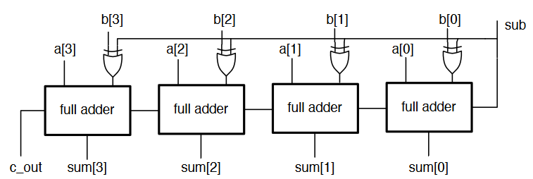
- In a synchronous system, we place the operands in registers and sum the registers
- The speed at which we can run the clock to update the registers depends on the propagation delay of the adder
- Can only clock the circuit as fast as the critical path allows
- In an adder, this is the carry from LSB to MSB
- Wider adders lengthen this period
Carry-Lookahead Adders
- A bit position generates a carry if it produces a carry, no matter what the carry in to that stage is
- A bit position propagates a carry if it produces a carry whenever it's carry is high
- This can be expressed as logical expressions
- The carry out of bit position is
- Also,
- The carry of each bit position can be expressed in terms of the previous ones
- At each stage, the sum, generate, and propagate can be computed
- This allows us to compute any intermediate carry bit
- Since and signals depend only on and , there is no more ripple
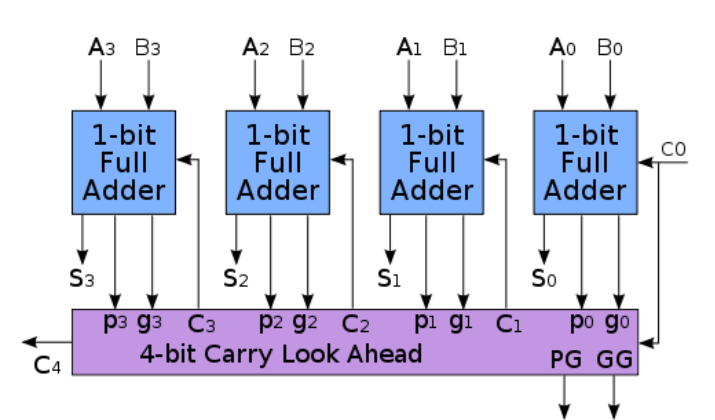
- Several can be chained to implement a much wider adder
- Wider lookahead require much more gates
- Instead of building wider adders from just gates, larger adders can be built up hierarchically from smaller adders (the and output signals are chained)
Other techniques for fast adders include carry-skip adders, which allow carries to skip over bits, and the Manchester carry chain, which uses shared logic for lookahead
Multipliers
- Binary multiplication is done similar to decimal long multiplication
- Multiplication between two bits is an and operation
- After each multiplication stage, one of the operands is shifted
- Partial products as the product of each pair of bits in each shift position are generated
- These partial products are then all summed
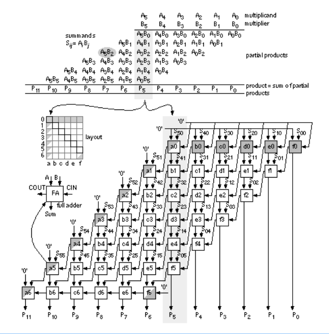
- Alternative architectures try to reduce the amount of addition, eg the Wallace multiplier
- FPGA tools take care of implementing multipliers efficiently using LUTs
- Wider multipliers are mapped to DSP blocks
- Very wide ones might use multiple DSPs
Fixed Point Arithmetic
Fixed point notation allows us to work with fractional numbers.
- Place a binary point at any location within the number
- Arithmetic is performed as integers
- The location of the binary point is kept track of
- Designer can select a precision suited to the application
The only difference when calculating a fixed point value is that some numbers have a weight that is a negative power of two, ie with a fixed point in the middle is .
-
The binary number now consists of two parts
- The integer part determines the range
- The fractional part determines the precision
-
Choosing a different position for the point allows trading accuracy for range
- 4 integer bits gives a range of 0-15
- 6 fractional bits can represent values with a precision of up to
-
There is no fixed notation for stating the position of a binary point, so it is important to be clear
- An bit fixed point number with fractional bits has integer bits
- If the number is signed, the first bit also has negative weight
-
Not all numbers can be represented exactly in a given fixed point format
- This causes some error, but selecting an appropriate precision for the use case can make this tolerable
- True also for floating point
Fixed Point Conversion
The easiest way to convert a fractional number to a given fixed point format is as follows:
- Multiply the number by where is the number of fractional bits
- Round the result to an integer
- Convert the integer to binary in the standard way
- Use the binary representation of that number as the fixed point representation
- Remember where the position of the binary point is for the calculation
For example, convert 2.384 to an 8 bit number with 6 fractional bits
- is the fixed point approximation
- is the actual value of the approximation
- The error is 0.006625 absolute or 0.28% relative
- Probably fine, depending upon the design
When converting, there are some things to watch out for:
- Need to maintain the same binary point position for all values
- If the converted number exceeds the width of the format then integer bits are lost
- Always work out the max integer width and precision you need first based on expected integer range
- When numbers are signed, the MSB has negative weight
Arithmetic affects the binary point:
- Addition and subtraction don't change the position, but an extra bit may be needed to prevent overflow
- Multiplication of an bit number with fractional bits and a but number with fractional bits yields an bit number with fractional bits
- It is important to keep track of where integer and fractional parts are in circuits
Fixed Point in Verilog
Verilog has no native support for fixed point, so the designer must keep track of the positions within the code. Vector slicing is used to choose the required bits. The module below multiplies two numbers with 4 integer and 12 fractional bits.
module mul_short(input signed [15:0] a,b, output signed [11:0] prod)
wire signed [31:0] x = a * b; //wider to prevent result being truncated
assign prod = x[31:20];
All verilog signals are treated as unsigned numbers by default, and we can use built in arithmetic operators on them.
Signed Arithmetic in Verilog
Any reg or wire is considered unsigned, unless it is declared as a signed signal
wire signed [3:0] x;
wire signed [15:0] y;
Signals like this are considered signed, and the design tools take care of generating signed circuits. For signed operations, all operands must be declared singed or verilog will default back to unsigned arithmetic. Signals can be cast using signed() and unsigned() functions
A basic 4-bit signed adder:
module add_signed(input signed [2:0] a,b, output signed [3:0] sum);
assign sum = a+b;
endmodule
A 3-bit signed adder with a carry out will be generated, and any sign-extension is done automatically.
Signed literals can also be used
reg signed [15:0] count_limit = -16’d47
reg signed [7:0] bits_left = 8’d12
When using unsigned vectors, verilog will automatically zero-extend when needed, which is bad for signed numbers. When declaring signals as being signed, verilog automatically sign-extends instead.
reg signed [15:0] x = 8'b1001_1111;
//results in x= 1111_1111_1001_1111
To mix signed and unsigned numbers, it is important to manually cast unsigned to signed:
module add_signed(input signed [2:0] a,b, input carry_in, output signed [3:0] sum);
assign sum = a + b + \$signed({1'b0, carry_in});
endmodule
carry_inis casted so signed circuitry is generated- It is extended with a
0because just casting a single bit to signed would result in a-1- This is important to do to prevent numbers becoming negative
A signed number can be truncated to narrow it's width, but only safely when the upper bits are all the same as the new MSB:
11110101safely truncates to10101(-11)000000011100safely truncates to011100(28)
Verilog will always truncate MSBs as needed if not careful, so care must always be taken when working with signed arithmetic
- Look out for synthesis warnings
- Make internal signals as wide as needed then truncate at the output
Floating Point
- Floating point allows to represent fractional numbers with an adjustable scale
- 32 bits are decomposed into separate fields that make up a number
| Sign | Exponent | Mantissa |
|---|---|---|
| 1 bit | 8 bits | 23 bits |
- Can represent numbers as small as and as large as
- Not all numbers can be accurately represented
- The exponent determines which powers of two the window of values covers
- The mantissa determines where within the window the value is
- As the size of the window increases, the less accurate the values can be
- Floating point circuits are large and complicated
- Not supported in most synthesis tools
- IP blocks are provided for floating point computation, but it should be considered how necessary it is before use
Timing & Pipelining
So far, digital circuits have been considered as instantaneous, where outputs are available immediately. This is an approximation, as there are delays in the propagation of signals through circuits. There are delays associated with many elements in circuits, and these need to be analysed and take in to account.
- Every gate or circuit element exhibits a propagation delay
- A change in the input causes a change in output, but only after a propagation delay:
- Delay arises due to low level factors to do with analog properties including capacitance
- Figures usually supplied by manufacturers
- Can differ for different gates
- Can be affected by temperature
- Low-to-high may differ from high-to-low delay
- Also related to fanout
- The number of inputs the output is driving
- This information can give the total propagation delay for a whole circuit
- Sum up all delays along all paths from inputs to outputs
- Worst case delay is the one we're concerned with
- Different path delays can cause internal glitches
- The worst case through a circuit is the deciding factor in how fast we can supply inputs
- Sum up all delays along all paths from inputs to outputs
Combinational Timing
It is typically easiest to trace through a circuit gate by gate, working out what the delay would be at each step. The gate delay can be indicated on timing diagrams, but only when specifically interested in them. The diagram shows a circuit, along with it's timing diagram including propagation delay.
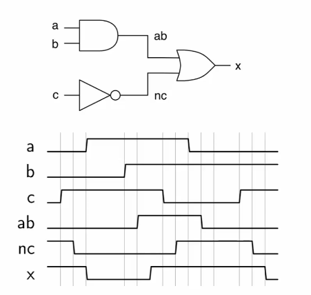
Attaching some numbers to the delays:
- ns
- ns
- ns
There are four inputs and one output in this circuit, so four possible paths. All paths have the same delay of 6ns.
Another example:
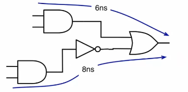
- The first two paths have a 6ns delay
- the second two paths also include an inverter, which adds another 2ns of delay for a total of 8ns
Looking again at the ripple adder, and assuming each gate has a unit delay:
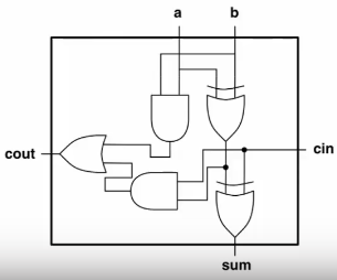
- a,b to sum has 2 delays
- cin to sum has 1 delay
- a,b to cout has 3 delays
- cin to cout has 2 delays
- Worst case is 3 delays, so this is how long we must wait for signals to propagate fully
Uneven path delays mean there may be invalid intermediate values before outputs settle, called glitches. It is important to wait for all signals to propagate to avoid incorrect results in the circuit.
The total delay of an n-stage ripple adder is gate delays:
- The 1st stage has 3 delays
- intermediate ripple stages have 2 delays
- The final stage will have 2 delays
Any combinational circuit element will have a delay, which can be determined from it's datasheet. Combining larger complex combinational elements must follow the same rules as combining gates. Consider the circuit to the right which computes :
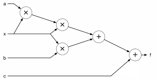
- The longest path from input to output is through the 2 multipliers and 2 adders
- Assuming 4ns and 2ns delay respectively, the total worst case delay is 12ns
Synchronous Timing
When composing large combinational circuits, the timing characteristics of each part must be considered to ensure that inputs and outputs are all timed correctly, analysing all paths. Any change to the circuit requires re-analysis of the timing behaviour. Sequential circuits are more complex to analyse.
- A synchronous system has a single clock that marks the timesteps when the new inputs are passed to sub-circuits
- At each rising edge, register outputs change
- Any combinational path must process this input, and have the result ready before the next clock cycle
- The clock must be slow enough to accommodate the slowest path between two flip-flops
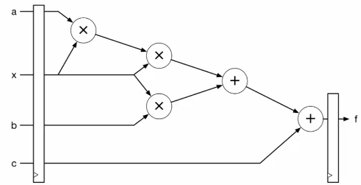
- At the first clock edge, values emerge from the first set of registers and propagate through the circuit, taking 12ns
- After 12ns, the values at the combinational output are stable and correct
- At the next clock edge, this output is stored in the register, and a new set of values enter the combinational circuit
- The maximum frequency = 1/12ns = approx 83MHz
- Or any slower clock will also work
When looking at a larger synchronous circuit:
- There will be a delay between any pair of registers
- The output of any register must have enough time to propagate through all the combinational logic to the next input
- The paths between all pairs of registers is considered, and the longest is selected as the critical path
- The critical path determines the maximum clock frequency for the whole circuit
Flip-Flop Timing
Recall how flip-flops are constructed, in a master/slave arrangement such that the master is active low and the slave active high, which traps data on the rising edge of the clock.
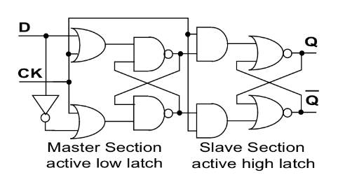
int represents the output of the master latch, and follows the input as long as clk is low. When clk is high the slave latch becomes transparent, passing through the trapped value.
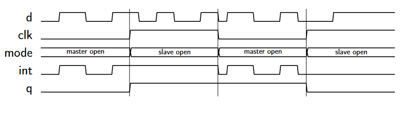
The actual timing characteristics are a little more complex:
- There is a clock-to-q delay, which is the delay between the clock edge and output changing
- Any desired input must arrive and be stable for a portion of time before the rising edge: the setup time
- The input must be held for a short while after the rising edge: the holdtime*
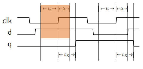
- For a more accurate max clock period, this must be factored in
- Min clock period is given by
- This does not factor in hold time
- The previous register must not produce an output that can reach the next register's input before after the rising edge
- As long as , this cannot happen
- is often 0 in modern devices
Example
Assuming a gate delay of 1ns, , and , determine the max clock frequency for a 6 bit ripple adder.
- bit ripple adder has gate delays
- For 6 bits, delay is 12ns
- Require
Synchronous Design
- When designing a circuit, we want to process large amounts of data
- Software programs used for data processing spend most of their time inside loops
- eg processing an image means applying a filter which involved maths over each pixel of the frame
- Combinational circuits with no clocks become difficult to build as they increase in size
- Difficult to keep track of the delay
- A synchronous system gives a predictable, fixed rate of data movement so the system can be modelled more easily
- I/O typically supplies data at a regular rate
- Sensors/ADCs
- I/O Busses such as PCIe
- Outputs read from a memory
- Building a data processing pipeline allows computation to be done quicker than a processor
- Can exploit parallelism
- Implement complex, custom datapaths
- Throughput is the number of input values that can be processed per unit time
- Determines the real speed of the circuit
- A fully synchronous circuit that can accept one set of inputs per cycle has a throughput of clock speed x amount of data per input
- Latency is the time between an input entering the system, and the computed output emerging from the system
- Less critical as it is a fixed delay
- Generally, it is desirable to maximise throughput, even if this comes at a slight cost of latency
- The limiting factor in any circuit is combinational propagation delay
- The largest chunk of combinational logic between any two registers determines the max frequency
- Large chunks of logic can be broken down by adding another register in the middle
- This increases latency, but allows the circuit to be clocked faster
Pipelining Circuits
Recall the polynomial calculation circuit from earlier. If another register stage is added in the middle, we now have two sets of paths between three registers:
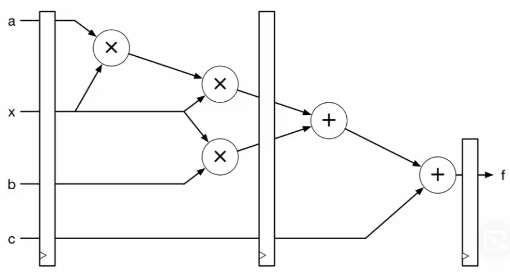
- The longest path between the first two register stages is through two multipliers: 8ns
- Longest path between second pair is 4ns
- Critical path is now 8ns, so can be clocked at 125MHz
- Latency is now 2 clock cycles, 16ns
- Throughput has been increased
This can be broken down further to add yet another register stage:
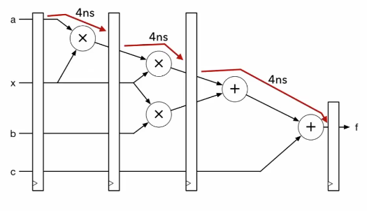
- Critical path now 4ns, clock speed now 250MHz
- Latency now 3 cycles (12ns)
- Have increased throughput and decrease latency
It would be pointless to add another stage between the two final adders as the critical path would still be elsewhere. It is important to place register stages to balance delays between pairs.
As a general rule, clock frequency can be increased by splitting up combinational logic. This is pipelineing
- A heavily pipeline circuit has many pipeline stages to allow the clock to be as fast as possible
- Even if cycle latency increases, may actually still be faster due to increased clock
- Leads to more complex designs and increased resource usage
To add a pipeline stage to a circuit:
- Find the largest block of combinational logic
- Break all paths between the registers with a new pipeline stage
- Wherever the break crosses a signal, place a register
- Registers are drawn combined but each signal requires a separate register
- Some registers will do nothing but delay signals so they align correctly
- The widths of registers will depend on the signals going in/out of them
Timing in FPGAs
- On FPGAs, logic is implemented in LUTs, so gate delays are not relevant
- A 6-input LUT can implement any function of 6 inputs
- The propagation delay is the same no matter what function is implements
- If a function is too large for a single LUTs, it will be spread accross multiple, increasing delay
- A single LUT in a Xilinx Virtex-6 is around 240ps
- Other FPGA resources have specified delays too
- DSP blocks have a specific combinational delay
- Registers can be enabled to decrease the critical path
- DSP blocks have a specific combinational delay
- Total combinational delay in an FPGA is composed of
- Logic delay: delay through LUTs, DSPs, etc
- Routing delay: the delay through the routing fabric
- Synthesis and mapping tools will break logic into blocks, but pipelining is done as coded in verilog
- Place and route tools will minimise routing delay
- Use numbers from datasheet to find critical paths
- FPGAs have many flip flops around the chip to allow deep pipelining
- Timing characteristics are given in datasheet
- A slice register has clock-to-output delay, , of around 0.4ns
- Setup and hold times are around 0.4ns and 0.2ns, respectively
- Specifics depend on which outputs are used
- Slice multiplexers affects timing
Interfaces
- FPGAs come in a wide variety of packages with a range of IO capabilities
- Most pins are reserved for specific uses such as voltage rails, clocks, configuration
- Other pins are multifunction and used for I/O
- FPGAs can be incorporated into a system in many ways
- Standalone, interfacing with peripherals and implementing all functionality
- As a peer to a more general purpose processor, connected with high bandwith
- As an accelerator on a high performance bus with shared memory
- As a separate device that communicates with another processor over a lower throughput bus
- How to integerate and communicate with an FPGA depends on the application
- Tightly coupled offers good bandwith but requires complex OS support
- Treating it as an accelerator like a GPU allows it to work with the CPU
- New hybrid FPGA designs that include an embedded processor in the same fabric
- Design built around a processor subsystem along with programmable logic
- High throughput interconnect
ADCs and DACs
- Interfacing with the real, analog world requires converting between analog and digital signals
- Analog-to-digital converters take an analog voltage level and convert it to a digital word
- Digital-to-analog converters take a digital word and convert to an analog voltage level
- ADCs and DACs are characterised by
- Sampling rate: the number of values the device can create/consume per second
- Determines the bandwidth based on the Nyquist theorem
- Resolution: the number of different levels the device can differentiate between
- Various fidelity characteristics such as linearity, noise, jitter
- Sampling rate: the number of values the device can create/consume per second
- In most cases, external ADCs/DACs are used with FPGAs
- Modern FPGAs include analog interfaces with internal ADCs
- Recent RFSoC radio-focused FPGAs include high speed ADCs and DACs on chip for integrated RF implementation
GPIO
- Most FPGAs and microcontrollers have pins for general purpose I/O
- Each pin can be set as an input or output for a single bit
- The I/O voltage level is customisable for banks of GPIO pins
- Easiest way to get data in and out of an FPGA
- Support switching rates of over 200MHz
- The number of pins is generally limited and insufficient for creating large parallel data busses
- Parallel I/O at high speeds requires detailed timing calibration and synchronisation
PWM
- Method of switching an output on and off, where the ratio of on to off, the duty cycle, gives an average output level
- Used for changing motor speed, servo direction, LED brightness
- Works due to the inertial load of output devices
- High speed switching means the overall output level is the average of the high and low periods
- An LED flickering at 500Hz cannot be detected as flickering by a human eye
- Microcontrollers use timers to generate waveforms, and the number of timers available limits the number of PWM signals that can be generated
- FPGAs can create counters specifically for PWM
module pwmgen #(parameter CNTR_BITS=6) (input clk, rst,
input [CNTR_BITS-1:0] duty,
output pwm_out);
reg [CNTR_BITS-1:0] pwm_step;
always @ (posedge clk) begin
if(rst)
pwm_step <= 1'b0;
else
pwm_step <= pwm_step + 1'b1;
end
assign pwm_out = (duty >= pwm_step);
endmodule
CNTR_BITSis the width of the counterdutyis the number of steps that the pwm signal is high forpwm_stepis the internal counter for each period
UART
- Universal Asynchronous Receiver/Transmitter is the easier way of sending multi-bit data between two systems
- Uses a single wire
- Asynchronous because no clock line between
- Baud rate is pre-agreed
- Data is transmitted in frames
- Frames can vary in bit length, and sometimes include parity, start, and stop bits
- Shift register is used at either end for parallel-serial conversion
- Rx of one device connected to Tx of another
- Combination of start and stop bit means frames can always be detected
- Can be issues when clocks are not well matched, which limits possible throughput
SPI
- Serial Peripheral Interface is a syncrhonous communication protocol that uses a shared clock at both transmitter and receiver
- Master initiates communication and generates clock
- Slave devices used as peripherals
- A single master can communicate with multiple slaves on the same SPI bus
- Four signals required
SCLK- the clock generated by the masterMISO- master in slave out- Data input from slave to master
MOSI- Data output from master to slave
SS- slave select- Select which slave is being communicated with
- Typically active low
- Each slave connected to a master requires a separate slave select line
- Master outputs the same clock for synchronous communication
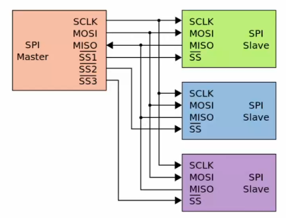
- To initiate communication, the master sets the required slave select line low and sends a clock signal
- On each clock edge, the data can be sent bi-directionally on
MOSIandMISO - With multiple slaves, the
MISOline must only be driven by one at a time so other slaves must be set to high impedance - All devices must agree on clock frequency, polarity and phase
- Specified in datasheets
I2C
- Inter-intergrated circuit protocol is similar do SPI but has different features
- Uses fewer wires due to lack of slave select lines
- Uses addressing to allow a large number of devices to share the same lines
- Only two wires
- SDA - serial data
- SCL - serial clock
- I2C clock is usually 100kHz
- All devices connected to an I2C bus act the same
- Whichever device is transmitting is the master for that communication
- Pull-up resistors keep each line high when no device is transmitting
- The device intending to communicate indicates this by pulling SDA low
- Data is then put onto the bus while SCL is low and sampled by slave devices during the rising edges
- Simpler signalling means more complicated data framing
- Pulled low to start
- 7 bit address sent
- 1 bit for read/write mode
- 1 bit slave ack
- 8 bit word
- 1 bit ack signal
- Stop bit
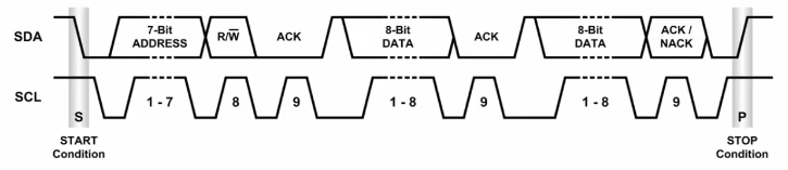
- Takes 20 cycles to read a single byte
- Vs 10 for SPI
- I2C is also half-duplex with a slow clock
- I2C used when there is less pins, SPI needed for higher data throughput
High Speed Serial I/O
- Higher speed communication off ship is facilitated by special serial/desrial blocks
- These take data words and serialise them, and transmit them over differential pairs of I/O pins
- Controller by high-speed clocks
- Can acheive up to 10s of gigabit speeds
- Differential signalling is used to improve noise resistance at high speed
- Signal sent twice, one an inverted copy of the other
- Balanced lines means better resistance to EM interference
- Clock information is encoded in data that is sent
- Data is encoded and scrambled to ensure sufficient transitions between 1s and 0s for receiver to be able to decode
- Extra bits are added to the data bits to ensure sufficient transitions and DC balance
- Specific schemes are specified by different physical layer standards
- 8b/10b means 2 extra bits are added to each byte
- Effective data rate is determined from two specifications
- Baud rate
- Encoding scheme
- For example, 2GHz with 8b/10b encoding gives 200MB/s
- 20% of baud rate is encoding overhead
- Multiple lanes are used to improve throughput
- PCIe gen 3 had a transfer rate of 8Gb/s per lane and uses a 128b/130b encoding
- 985 MB/s
- 1.5% encoding overhead
- 16 lanes (PCIe3 x16) gives about 16GBps
- PCIe gen 3 had a transfer rate of 8Gb/s per lane and uses a 128b/130b encoding
- Use in many interfaces
- Serial ATA for disks and storage
- Gigabit ethernet
- Used over a variety of physical media
- Circuits required to interface with high speed I/O have to be designed carefully to meet strict timing requirements
- Vendors usually provide IP for this
- IP blocks designed to specific standard for the interface they are meant to be using
- The simplest form of communicating between modules in design is the ready/valid handshaking
- One module is a source, another a sink
- The sink module asserts a ready signal when it is ready to consume data
- The source module asserts a valid signal when it is outputting valid data
- At any clock edge when both ready and valid are asserted, data is transferred on the data line
- Can introduce a bottleneck
- In the source module, the pipeline can be halted when the sink is not ready, and resumed when ready
- In the sink, ready is asserted when data is ready to be accepted
- Such an interface allows a FIFO buffer to be inserted between modules to offer more isolation
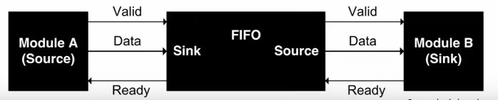
AXI4
- Most hybrid FPGAs include an ARM processor
- Advanced microcontroller bus architecture (AMBA) is an on-chip interconnect specification introduced by ARM for use in SoCs
- Defines a number of interfaces
- AXI4 for high performance memory mapped communication
- AXI4-Lite is a simpler interface for low throughput
- AXI4-Stream is for high speed streaming data
- Reads are initiated by a master over the read address channel
- The slave response with data over the read data channel
- Writes are similar, with address and control data being placed on the write address channel
- The master sends data over the write data channel
- Slave responds on the write response channel
- Read and write channels are separeatre, allowing bidirectional communication
- AXI4 supports bursts of up to 256 words
- Each master/slave pair can have a separate clock
- A system consists of multiple masters and slaves connected on an interconnect
- Most vendor IP is provided with an AXI4 interface to simplify integration into a design
- Different interface specifications are shown in datasheets
Processor Implementation
Fixed Purpose Processors
- Digital circuits designed to implement a specific application, when fabricated so silicon, are Application Specific Integrated Circuits (ASICs).
- The alternative is creating FPGA bitstreams and loading them into FPGAs
- Changing the function of an FPGA is easy, creating new ASICs is expensive.
Custom datapaths for specific applications have the benefit of high performance due to being tailored for the use case, and being able to exploit parallelism. When repeating the same computation on a stream of data, a simple feed forward datapath is most performant, and can be pipelined to improve throughput
The example below shows a feed-forward data path for multiplying two complex numbers, with six pipeline stages.
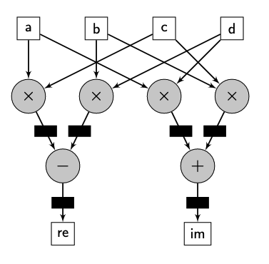
Finite Impulse Response (FIR) filters are also easy to map to hardware. The delay blocks are just registers, and the arithmetic blocks are implemented directly. Using the transpose form shortens the critical path to improve performance further.
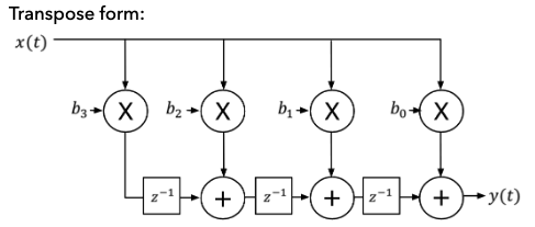
General Purpose Processors
General purpose processors need to support:
- A set of arithmetic operations
- Movement of data in and out of arithmetic logic
- A way of breaking down functions into discrete steps
- A way to program the circuit to carry out the steps
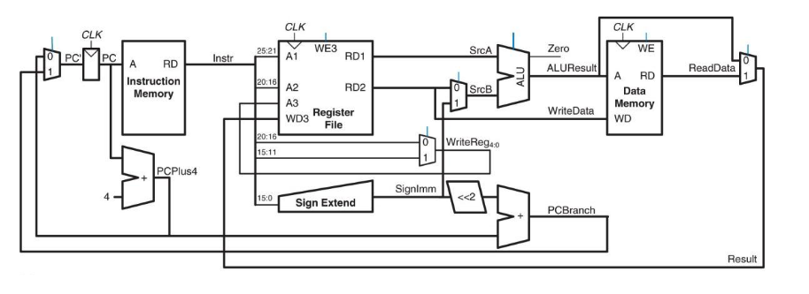
Each of these components can be constructed in Verilog using basic synchronous elements.
Program Counter
Just a register with an input and output (32 bits).
module pc_reg(input clk, rst, input [31:0] pcnext, output reg [31:0] pc);
always @ (posedge clk) begin
if (rst) //point to base address on reset
pc <= 32'd0;
else
ps <= pcnext;
end
endmodule
Register File
The register file constains 32 32-bit registers, and has two read ports.
- Two read address, one for each port (
ra1,ra2) - A write address (
wa3) - A write data input (
wd3) - Two read outputs (
rd1,rd2) - A write enable input (
we3)
module regfile (input clk, we3,
input [4:0] ra1, ra2, wa3,
input [31:0] wd3,
output [31:0] rd1, rd2);
reg [31:0] rf [0:31];
always @ (posedge clk) begin
if(we3) rf[wa3] <= wd3;
end
assign rd1 = (ra1 != 32’d0) ? rf[ra1] : 0;
assign rd2 = (ra2 != 32’d0) ? rf[ra2] : 0;
endmodule
RAM
- Standard memory with one read and one write port
- Reads are combinational and writes synchronous
module dmem (input clk, we,
input [31:0] ad, wd,
output [31:0] rd);
reg [31:0] ram [0:65535];
// byte-addressing to word-aligned
always @ (posedge clk)
if(we) ram[ad[31:2]] <= wd;
assign rd = ram[ad[31:2]];
endmodule
Combinational elements
There are other combinational elements in the processor, multiplexers, incrementers, sign extension, etc, all of which are fairly easy to implement. The ALU may be more complex, but a simple example of one is shown below, which supports 8 different functions, selected using a function control input F[2:0].
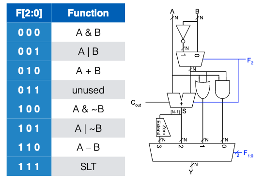
module alu (input [31:0] a,b, input [2:0] func,
output reg [31:0] out);
wire [31:0] bfin = func[2] ? ~b : b;
wire [31:0] sumout = a + bfin + func[2];
always @ *
case (func[1:0])
2'b00: out = a & bfin;
2'b01: out = a | bfin;
2'b10: out = sumout;
2'b11: out = sumout[31];
endcase
endmodule
Processor control
The processor also has a control unit, which asserts signals to inform the datapath for the processing of a particular instruction. The control unit uses combinational logic to break down the instruction and then output signals to control the rest of the processor
Pipelining
A pipeline processor requires register stages to be added within the data and control paths.
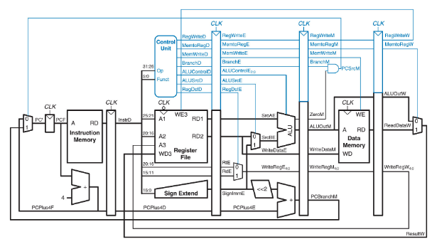
ES3C5 - Signal Processing
Brief Notes + Equations
This is just a collection of notes for ES3C5 Signal Processing that I have found useful to have on hand and easily accessible.
The notes made by Adam (MO) cover everything so this is just intended to be an easy to search document.
Download lecture notes here
Use ./generateTables.sh ../src/es2c5/brief-notes.md in the scripts folder.
| Laplace Conversion | |
|---|---|
| Laplace Table | Insert table here |
| Finding Time Domain Output | |
| Input as Delta Function | |
| Input as Step Function | |
| LTI System Properties | LTI = |
| 3 - Poles and Zeros | |
|---|---|
| General Transfer Function as 2 polynomials | |
| Factorised Transfer Function | |
| Real system as real | |
| Zero Definition | Roots z of the numerator. When any , |
| Pole Definition | Poles p of the denominator. When any , approaches |
| Transfer Function Gain | K is the overall transfer function gain. (Coefficient of and is 1.) |
| Stable System | A system is considered stable if its impulse response tends to zero or a finite ... |
| Components to Response | Real Components Exponential Response Imaginary angular f... |
| 4 - Analog Frequency Response | |
|---|---|
| Frequency Response | Frequency response of a system = output in response to sinusoid input of unit ma... |
| Continuous Fourier Transform | |
| Inverse Fourier Transform | |
| Magnitude of Frequency Response (MFR) | |
| Phase Angle of Frequency Response (PAFR) - | |
| Phase Angle of Frequency Response (PAFR) - |
| 5 - Analog Filter Design | |
|---|---|
| Ideal Filters | Each ideal filter has unambiguous |
| Realisability | System starts to respond to input before input is applied. Non-zero for . |
| Causality | Output depends only on past and current inputs, not future inputs. |
| Realising Filters | Realise as we seek smooth behaviour. |
| Gain (linear dB) | |
| Gain (dB linear) | |
| Transfer Function of Nth Order Butterworth Low Pass Filter | |
| Frequency Response of common Low pass Butterworth filter | |
| Normalised Frequency Response of common Low pass Butterworth filter | |
| Minimum Order for Low Pass Butterworth | |
| Low pass Butterworth Cut-off frequency (Pass) | |
| Low pass Butterworth Cut-off frequency (Stop) |
| 8 - Signal Conversion between Analog and Digital | |
|---|---|
| Digital Signal Processing Workflow | See diagram: |
| Sampling | Convert signal from continuous-time to discrete-time. Record amplitude of the an... |
| Oversample | Sample too often, use more complexity, wasting energy |
| Undersample | Not sampling often enough, get |
| Aliasing | Multiple signals of different frequencies yield the same data when sampled. |
| Nyquist Rate | |
| Quantisation | The mapping of |
| Data Interpolation | Convert digital signal back to analogue domain, reconstruct continous signal fro... |
| Hold Circuit | Simplest interpolation in a DAC, where amplitude of continuous-time signal match... |
| Resolution | |
| Dynamic range |
| 9 - Z-Transforms and LSI Systems | |
|---|---|
| LSI Rules | Linear Shift-Invariant |
| Common Components of LSI Systems | For digital systems, only need 3 types of LSI circuit components. |
| Discrete Time Impulse Function | Impulse response is very similar in digital domain, as it is the system output w... |
| Impulse Response Sequence | |
| LSI Output | |
| Z-Transform | |
| Z-Transform Examples | Simple examples... |
| Binomial Theorem for Inverse Z-Transform | |
| Z-Transform Properties | Linearity, Time Shifting and Convolution |
| Sample Pairs | See example |
| Z-Transform of Output Signal | |
| Finding time-domain output of an LSI System | Transform, product, inverse. |
| Difference Equation | Time domain output directly as a function of time-domain input as ... |
| Z-Transform Table | See table... |
| 10 - Stability of Digital Systems | |
|---|---|
| Z-Domain Transfer Function | |
| General Difference Equation | |
| Poles and Zeros of Transfer Function | |
| Bounded Input and Bounded Output (BIBO) Stability | Stable if bounded input sequence yields bounded output sequence. |
| 11 - Digital Frequency Response | |
|---|---|
| LSI Frequency Response | Output in response to a sinusoid input of unit magnitude and some specified freq... |
| Discrete-Time Fourier Transform (DTFT) - Digital Frequency Response | |
| Inverse Discrete-Time Fourier Transform (Inverse DTFT) | |
| LSI Transfer Function | |
| Magnitude of Frequency Response (MFR) | |
| Phase Angle of Frequency Response (PAFR) - | |
| Example 11.1 - Simple Digital High Pass Filter | See image... |
| 12 - Filter Difference equations and Impulse responses | |
|---|---|
| Z-Domain Transfer Function | |
| General Difference Equation | |
| Example 12.1 Proof y[n] can be obtained directly from H[z] | See image... |
| Order of a filter | |
| Taps in a filter | Minimum number of unit delay blocks required. Equal to the order of the filter. |
| Example 12.2 Filter Order and Taps | See example... |
| Tabular Method for Difference Equations | Given a difference equation, and its input x[n], can write specific output y[n] ... |
| Example 12.3 Tabular Method Example | See example |
| Infinite Impulse Response (IIR) Filters | IIR filters have |
| Example 12.4 IIR Filter | See example |
| Finite Impulse Response (FIR) Filters | FIR Filter are none recursive (ie, no feedback components), so a[k] = 0 for k!=0... |
| FIR Difference Equation | |
| FIR Transfer function | |
| FIR Transfer Function - Roots | |
| FIR Stability | FIR FILTERS ARE ALWAYS STABLE. As in transfer function, all M poles are all on t... |
| FIR Linear Phase Response | Often have a linear phase response. The phase shift at the output corresponds to... |
| FIR Filter Example | See example 12.5 |
| Ideal Digital Filters | Four main types of filter magnitude responses (defined over $0 \le \Omega \le \p...$ |
| Realising Ideal Digital Filters | Use poles and zeros to create simple filters. Only need to consider response ove... |
| Example 12.6 - Simple High Pass Filter Design | See diagram |
| 13 - FIR Digital Filter Design | |
|---|---|
| Discrete Time Radial Frequency | |
| Realising Ideal Digital Filter | Aim is to get as close as possible to |
| Practical Digital Filters | Good digital low pass filter will try to realise the (unrealisable) ideal respon... |
| Windowing | Window Method - design process: start with ideal and windowing infinite... |
| Windowing Criteria | |
| Practical FIR Filter Design Example 13.2 | See example... |
| Specification for FIR Filters Example 13.3 | See example... |
| 14 - Discrete Fourier Transform and FFT | |
|---|---|
| Discrete Fourier Transform DFT | |
| Inverse DFT | $x[n] = \frac{1}{N}\sum_{k=0}^{N-1}X[k]e^{jnk\frac{2\pi}{N}}, \quad n=\left { 0,1,2, \cdots , N-1 \right }$ |
| Example 14.1 DFT of Sinusoid | See example |
| Zero Padding | Artificially increase the length of the time domain signal by adding zero... |
| Example 14.2 Effect of Zero Padding | See example |
| Fast Fourier Transform FFT | Family of alogrithms that evaluate DFT with complexity of compare... |
| 16 - Digital vs Analogue Recap | |
|---|---|
| Aperiodic (simple periodic) continuous-time signal f(t) | Laplace, fourier transform. |
| More Complex Continuous-time signal f(t) | Fourier series, multiples of fundamental, samples of frequency response. |
| Discrete-time signal f[n] (infinite length) | Z-Domain, Discrete-time fourier transform |
| Discrete-time signal f[n] (finite length) | Finite Length N, convert to frequency domain (DFT), N points distributed over 2 ... |
| Stability | S-domain: negative real component, Z domain: poles within unit circle. |
| Bi-Linearity | Not core module content. |
| 17 - Probabilities and random signals | |
|---|---|
| Random Variable | A quantity that takes a non-deterministic values (ie we don't know what the valu... |
| Probability Distribution | Defines the probability that a random variable will take some value. |
| Probability Density Function (PDF) - Continuous random variables | |
| Probability mass function (PMF) - Discrete random variables | |
| Moments | |
| Uniform Distribution | Equal probability for a random variable to take any value in its domain, ie over... |
| Bernoulli | Discrete probability distribution with only 2 possible values (yes no, 1 0, etc)... |
| Gaussian (Normal) Distribution | Continuous probability distribution over , where values closer... |
| Central Limit Theorem (CLT) | Sum of independent random variables can be approximated with Gaussian distributi... |
| Independent Random Variables | No dependency on each other (i.e., if knowing the value of one random variable g... |
| Empirical Distributions | Scaled histogram by total number of samples. |
| Random Signals | Random variables can appear in signals in different ways, eg: |
| 18 - Signal estimation | |
|---|---|
| Signal Estimation | Signal estimation, refers to estimating the values of parameters embedded in a s... |
| Linear Model | See equation |
| Generalised Linear From | See equation |
| Optimal estimate | See equation |
| Predicted estimate | See equation |
| Observation Matrix | See below |
| Mean Square Error (MSE) | See equation |
| Example 18.1 | See example |
| Example 18.2 | See example |
| Linear Regression | |
| Weighted Least Squares Estimate | Weighted least squares, includes a weight matrix W, where each sample associated... |
| Maximum Likelihood Estimation (MLE) | See equation |
| 19 - Correlation and Power spectral density | |
|---|---|
| Correlation | Correlation gives a measure of time-domain similarity between two signals. |
| Cross Correlation | |
| Example 19.1 - Discrete Cross-Correlation | See example |
| Autocorrelation | Correlation of a signal with itself, ie or |
| Example 19.2 - Discrete Autocorrelation | See example |
| Example 19.3 - Correlation in MATLAB | See example |
| 20 - Image Processing | |
|---|---|
| Types of colour encoding | Binary (0, 1), Indexed (colour map), Greyscale (range 0->1), True Colour (RGB) |
| Notation | See below |
| Digital Convolution | |
| Example 20.1 - 1D Discrete Convolution | See example |
| Example 20.2 - Visual 1D Discrete Convolution | See example |
| Image Filtering | Determine output y[i][j] from input x[i][j] through filter (kernel) h[i][j] |
| Edge Handling | Zero-padding and replicating |
| Kernels | Different types of kernels. |
| Example 20.3 - Image Filtering | See example |
Part 1 - Analogue Signals and Systems
Laplace Conversion
Laplace Table
Insert table here

Finding Time Domain Output
- Transform and into Laplace domain
- Find product
- Take inverse Laplace transform
Input as Delta Function
Then , so .
Input as Step Function
Then , so .
LTI System Properties
LTI = Linear Time Invariant.
- LTI systems are linear. Given system and signals , etc
- LIT is Additive:
- LTI is scalable (or homogeneous)
- LTI is time-invariant, ie, if output then:
3 - Poles and Zeros
General Transfer Function as 2 polynomials
Factorised Transfer Function
Is factorised and rewrite as a ratio of products:
Real system as real
Where the numerator i a th order polynomial with coefficients s and the denominator is a th order polynomial with coefficients s. For a system to be real, the order of the numerator polynomial must be no greater than the order of the denominator polynomial, ie: .
Zero Definition
Roots z of the numerator. When any ,
Pole Definition
Poles p of the denominator. When any , approaches
Transfer Function Gain
K is the overall transfer function gain. (Coefficient of and is 1.)
Stable System
A system is considered stable if its impulse response tends to zero or a finite value in the time domain.
Requires all real components to be negative (on the left hand side of the complex s-plane of a pole-zero plot (left if the imaginary s axis)).
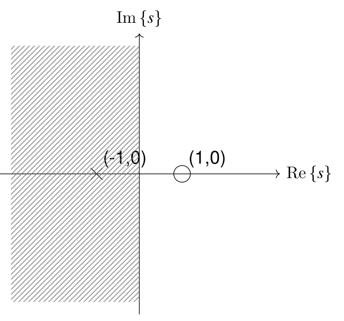
Components to Response
Real Components Exponential Response Imaginary angular frequency of oscillating responses.
4 - Analog Frequency Response
Frequency Response
Frequency response of a system = output in response to sinusoid input of unit magnitude and specified frequency, . Response is measured as magnitude and phase angle.
Continuous Fourier Transform
Laplace transform evaluated on the imaginary s-axis at some frequency .
radial frequency,
Inverse Fourier Transform
Magnitude of Frequency Response (MFR)
In words, the magnitude of the frequency response (MFR) is equal to the gain multiplied by the magnitudes of the vectors corresponding to the zeros, divided by the magnitudes of the vectors corresponding to the poles.
Phase Angle of Frequency Response (PAFR) -
Phase Angle of Frequency Response (PAFR) -
In words, the phase angle of the frequency response (PAFR) is equal to the sum of the phases of the vectors corresponding to the zeros, minus the sum of the phases of the vectors correspond to the poles, plus if the gain is negative.
Each phase vector is measured from the positive real s-axis (or a line parallel to the real s-axis if the pole or zero is not on the real s-axis).
5 - Analog Filter Design
Ideal Filters
Each ideal filter has unambiguous pass bands, which are ranges of frequencies that pass through the system without distortion, and stop bands, which are ranges of frequencies that are rejected and do not pass through the system without significant loss of signal strength. The transition band between stop and pass bands in ideal filters has a size of 0; transitions occur at single frequencies.
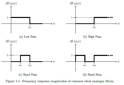
Realisability
System starts to respond to input before input is applied. Non-zero for .
Causality
Output depends only on past and current inputs, not future inputs.
Realising Filters
Realise as we seek smooth behaviour.
- Drop for ()
- Would not get suitable behaviour in frequency domain, as discarded 50% of system energy
- But can tolerate delays
- So shift sinc to the right
- Time domain shift = scaling by complex exponential in laplace
- True in fourier transform, so delay in time maintains magnitude but changes phase of frequency response
- Truncate
- As can't wait for infinity, so truncate impulse response.
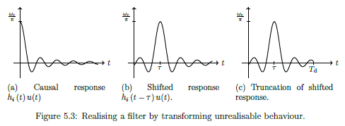
Gain (linear dB)
Gain (dB linear)
Transfer Function of Nth Order Butterworth Low Pass Filter
Butterworth = Maximally flat in pass band (freq response magnitudes are flat as possible for given order)
- = nth pole
- =
- =
- Form semi-circle to left of imaginary s-axis
- = half-power cut-off frequency
- Frequency where filter gain is or
Frequency Response of common Low pass Butterworth filter
Increasing order improves approximation of ideal behaviour
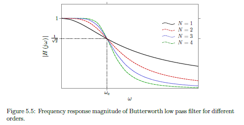
Normalised Frequency Response of common Low pass Butterworth filter
To convert normalised frequency form to non-normalised = multiply by the actual
Minimum Order for Low Pass Butterworth
Round up as want to over-satisfy not under-satisfy
Low pass Butterworth Cut-off frequency (Pass)
Gain in dB
Low pass Butterworth Cut-off frequency (Stop)
Gain in dB
6 - Periodic Analogue Functions
Exponential Representation from Trigonometric representation
Trigonometric from exponential - Real (cos)
Trigonometric from exponential - Imaginary (cos)
Fourier Series
Period signal = sum of complex exponentials.
Fundamental frequency , such that all frequencies in signal are multiples of .
Fundamental period
Fourier spectra only exist at harmonic frequencies (ie integer multiples of fundamental frequency)
Fourier Coefficients
Important property of Fourier series is how is represents real signals .
- Even magnitude spectrum
- Odd phase spectrum =
Fourier Series of Periodic Square Wave (Example)
Where
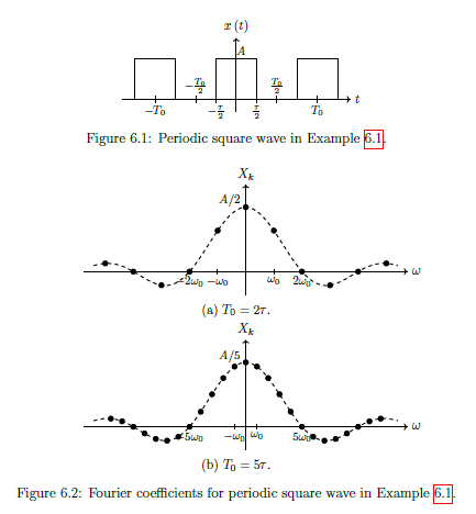
Output of LTI system from Signal with multiple frequency components
Or in other words:
The output of an LTI system due to a signal with multiple frequency components can be found by superposition of the outputs due to the individual frequency components. IE system will change amplitude and phase of each frequency in the input.
Filtering Periodic Signal (Example 6.2)
See example 6.2 below...
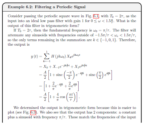
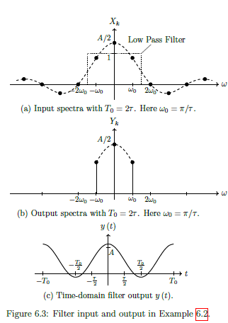
7 - Computing with Analogue Signals
This topic isn't examined as it is MATLAB
8 - Signal Conversion between Analog and Digital
Digital Signal Processing Workflow
See diagram:
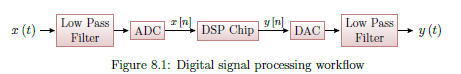
- Low pass filter applied to time-domain input signal to limit frequencies
- An analogue-to-digital converter (ADC) samples and quantises the continuous time analogue signal to convert it to discrete time digital signal .
- Digital signal processing (DSP) performs operations required and generates output signal .
- A digital-to-analogue converter (DAC) uses hold operations to reconstruct an analogue signal from
- An output low pass filter removes high frequency components introduced by the DAC operation to give the final output .
Sampling
Convert signal from continuous-time to discrete-time. Record amplitude of the analogue signal at specified times. Usually sampling period is fixed.
Oversample
Sample too often, use more complexity, wasting energy
Undersample
Not sampling often enough, get aliasing of our signal (multiple signals of different frequencies yield the same data when sampled.)
Aliasing
Multiple signals of different frequencies yield the same data when sampled.
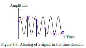
If we sample the black sinusoid at the times indicated with the blue marker, it could be mistaken for the red dashed sinusoid. This happens when under-sampling, and the lower signal is called the alias. The alias makes it impossible to recover the original data.
Nyquist Rate
Minimum ant-aliasing sampling Frequency.
Frequencies above this remain distinguishable.
Quantisation
The mapping of continuous amplitude levels to a binary representation.
IE: bits then there are quantisation levels. ADC Word length .
Continuous amplitude levels are approximated to the nearest level (rounding). Resulting error between nearest level and actual level = quantisation noise
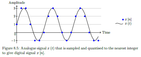
Data Interpolation
Convert digital signal back to analogue domain, reconstruct continous signal from discrete time series of points.
Hold Circuit
Simplest interpolation in a DAC, where amplitude of continuous-time signal matches that of the previous discrete time signal.
IE: Hold amplitude until the next discrete time value. Produces staircase like output.
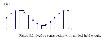
Resolution
Space between levels, often represented as a percentage.
For -bit DAC, with uniform levels
Dynamic range
Range of signal amplitudes that a DAC can resolve between its smallest and largest (undistorted) values.
9 - Z-Transforms and LSI Systems
LSI Rules
Linear Shift-Invariant
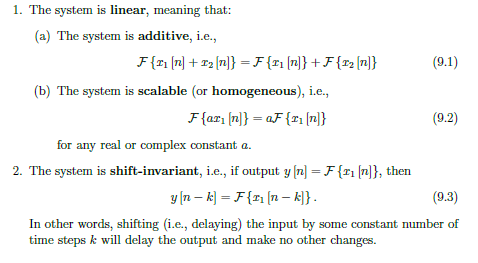
Common Components of LSI Systems
For digital systems, only need 3 types of LSI circuit components.
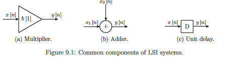
- A multiplier scales the current input by a constant, i.e., .
- An adder outputs the sum of two or more inputs, e.g., .
- A unit delay imposes a delay of one sample on the input, i.e, .
Discrete Time Impulse Function
Impulse response is very similar in digital domain, as it is the system output when the input is an impulse.
Impulse Response Sequence
LSI Output
Discrete Convolution of input signal with the impulse response.
Z-Transform
Converts discrete-time domain function into complex domain function , in the z-domain Assume is causal, ie
Discrete time equivalent to Laplace Transform. However can be written by direct inspection (as have summation instead of intergral). Inverse equally as simple.
Z-Transform Examples
Simple examples...
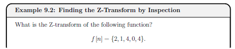
Binomial Theorem for Inverse Z-Transform
Cannot always find inverse Z-tranform by immediate inspection, in particular if the Z-transform is written as a ratio of polynomials of z. Can use Binomial theorem to convert into single (sometimes infinite length) polynomial of
Z-Transform Properties
Linearity, Time Shifting and Convolution
![]()
Sample Pairs
See example
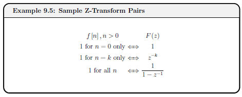
Z-Transform of Output Signal
Where = Pulse Transfer Function (as it is also the system output when the time-domain input is a unit impulse.) but by convention can refer to as the Transfer Function
Finding time-domain output of an LSI System
Transform, product, inverse.
- Transform and into z-domain
- Find product
- Taking the inverse Z-transform of
Difference Equation
Time domain output directly as a function of time-domain input as well as previous time-domain outputs (ie can be feedback).
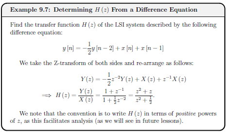
Z-Transform Table
See table...
![]()
![]()
10 - Stability of Digital Systems
Z-Domain Transfer Function
Negative powers of z.
No constraint on and to be real (unlike analogue) but often assume
General Difference Equation
Poles and Zeros of Transfer Function
- Coefficient of each in this form is 1.
- Poles and zeros carry same meaning as analogue
- Unfortunately symbol for variable and zeros are very similar (take care)
- Insightful to plot
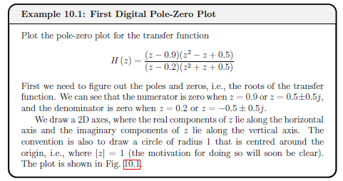
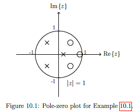
Bounded Input and Bounded Output (BIBO) Stability
Stable if bounded input sequence yields bounded output sequence.
A system is BIBO stable if all of the poles lie inside the unit circle
A system is Conditionally stable if there is atleast 1 pole directly on the unit circle.
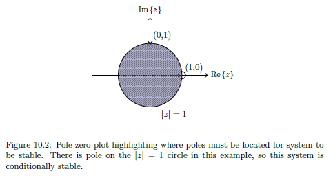
Explanation:
- An input sequence is bounded if each element in the sequence is smaller than some value .
- An output sequence corresponding to is bounded if each element in the sequence is smaller than some value .
11 - Digital Frequency Response
LSI Frequency Response
Output in response to a sinusoid input of unit magnitude and some specified frequency. Shown in two plots (magnitude and phase) as a function of input frequency.
Discrete-Time Fourier Transform (DTFT) - Digital Frequency Response
Where angle is the angle of th unit vector measured from the positive real -axis. Denotes digital radial frequency, measured in radians per sample
as spectrum of (frequency response).
Convention of writing DTFT includes or simply
Derivation: Using Z-Transform Definition.
Let be polar coords (), ie magnitude to r, angle . Hence rewrite
Then let , so that any point lies on the unit circle.
Inverse Discrete-Time Fourier Transform (Inverse DTFT)
LSI Transfer Function
is a function of vectors from the system's poles and zeros to the unit circle at angle .Thus from pole-zero plot, can geometrically determine magnitude and phase of frequency response.
Magnitude of Frequency Response (MFR)
In words, the magnitude of the frequency response (MFR) is equal to the gain multiplied by the magnitudes of the vectors corresponding to the zeros, divided by the magnitudes of the vectors corresponding to the poles.
Repeats every as Eulers Formula. Due to symettery of poles and zeros about real -axis, frequency response is symmetric about , so only need to find over one interval of
Phase Angle of Frequency Response (PAFR) -
In words, the phase angle of the frequency response (PAFR) is equal to the sum of the phases of the vectors corresponding to the zeros, minus the sum of the phases of the vectors correspond to the poles, plus if the gain is negative.
Repeats every as Eulers Formula. Due to symettery of poles and zeros about real -axis, frequency response is symmetric about , so only need to find over one interval of
Example 11.1 - Simple Digital High Pass Filter
See image...
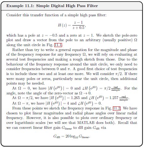
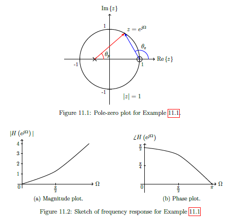
12 - Filter Difference equations and Impulse responses
Z-Domain Transfer Function
General Difference Equation
Real coefficients and are the same. (Note = 1, so no coefficient corresponding to ).
Easier to convert directly between transfer function (with negative powers of z) and the difference equation for output , ideal for implementation of the system. (rather than use time-domain impulse response )
Example 12.1 Proof y[n] can be obtained directly from H[z]
See image...
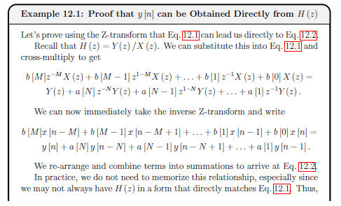
Order of a filter
Taps in a filter
Minimum number of unit delay blocks required. Equal to the order of the filter.
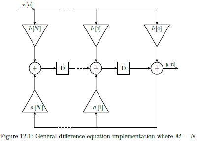
Example 12.2 Filter Order and Taps
See example...
Tabular Method for Difference Equations
Given a difference equation, and its input x[n], can write specific output y[n] using tabular method.
- Starting with input , make a column for every input and output that appears in difference equation
- ASsume every output and delayed input is initially zero (ie the filter is causal, initially no memory, hence system is quiescent)
- Fill in column for with given system input for all rows needed, and fill in delayed versions of
- Evaluate from inital input, and propagate the value of y[0] to delayed outputs (as relavent)
- Evaluate from s and
- Continue evaluating output and propagating delayed outputs.
Can be alternative method for finding time-domain impulse response
Example 12.3 Tabular Method Example
See example
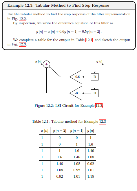
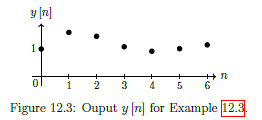
Infinite Impulse Response (IIR) Filters
IIR filters have infinite length impulse responses because they are recursive (ie feedback terms associated with non-zero poles in transfer function, hence exists.)
Standard transfer function and difference equation can be used to represent.
Not possible to have a linear phase response (so there are different delays associated with different frequencies, and they are not always stable (depending on the exact locations of poles.))
IIR filters are more efficient than FIR designs at controlling gain of response.
Although response is technically infinite, in practice decays towards zero or can be truncated to zero (assume response is beyond some value )
Example 12.4 IIR Filter
See example
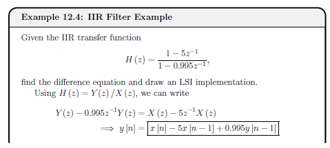
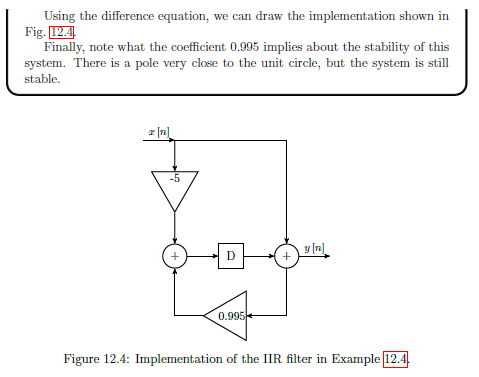
Finite Impulse Response (FIR) Filters
FIR Filter are none recursive (ie, no feedback components), so a[k] = 0 for k!=0.
Finite in length, and strictly zero beyond that ( for ). Therefore the number of filter taps dictates the length of an FIR impulse response
Since there is no feedback, can write impulse response as:
FIR Difference Equation
FIR Transfer function
Simplified from general differernce equation tranfer function.
FIR Transfer Function - Roots
More convenient to work with positive powers of z, so multiply top and bottom by then factor.
FIR Stability
FIR FILTERS ARE ALWAYS STABLE. As in transfer function, all M poles are all on the origin (z =0) and so always in the unit circle.
FIR Linear Phase Response
Often have a linear phase response. The phase shift at the output corresponds to a time delay.
FIR Filter Example
See example 12.5
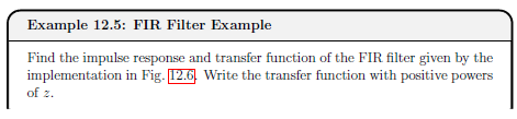
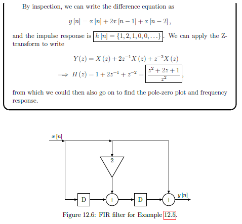
Ideal Digital Filters
Four main types of filter magnitude responses (defined over , mirrored over and repeated every )
- Low Pass - pass frequencies less than cut-off frequency and reject frequencies greater.
- High Pass - rejects frequencies less than cut-off frequency and pass frequencies greater.
- Band Pass - Passes frequency within specified range, ie between and , and reject frequencies that are either below or above the band within
- Band Stop - Rejects frequency within specified range, ie between and , and passes all other frequencies within
Ideal response appear to be fundamentally different from ideal analogue, however we only care over fundamental band where behaviour is identical
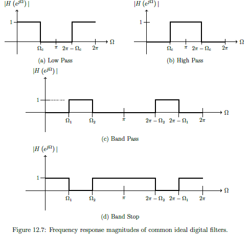
Realising Ideal Digital Filters
Use poles and zeros to create simple filters. Only need to consider response over the fixed band.
Key Concepts:
-
To be physically realisable, complex poles and zeros need to be in conjugate pairs
-
Can place zeros anywhere, so will often place directly on unit circle when frequency / range of frequency needs to be attenuated
-
Poles on the unit circle should generally be avoided (conditionally stable). Can try to keep all poles at origin so can be FIR, otherwise IIR, so feedback. Poles used to amplify response in the neighbourhood of some frequency.
-
Low Pass - zeros at or near , poles near which can amplify maximum gain, or be used at a higher frequency to increase size of pass band.
-
High Pass - literally inverse of low pass. Zeros at or near , poles near which can amplify maximum gain, or be used at a lower frequency to increase size of pass band.
-
Band Pass - Place zeros at or near both and ; so must be atleast second order. Place pole if needed to amplify the signal in the neighbourood of the pass band.
-
Band Stop - Place zeros at or near the stop band. Zeros must be complex so such a filter must be atelast second order. Place poles at or near both and if needed.
Example 12.6 - Simple High Pass Filter Design
See diagram
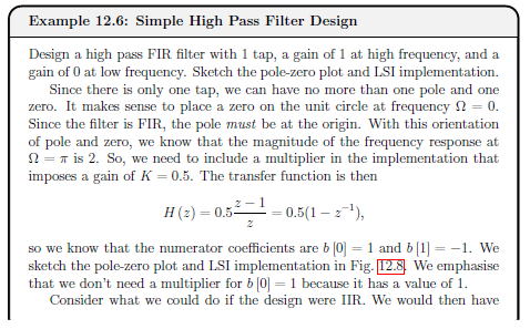
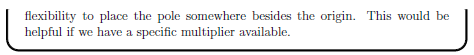
13 - FIR Digital Filter Design
Discrete Time Radial Frequency
As long as - otherwise there will be an alias at a lower frequency. So to avoid aliasing.
Realising Ideal Digital Filter
Aim is to get as close as possible to ideal behaviour. But when using Inverse DTFT, the ideal impulse response is .
This is analogous to the inverse Fourier transform of the ideal analogue low pass frequency response.
Sampled a scaled sinc function, non-zero values for . So needs to respond to an input before the input is applied, thus unrealisable.
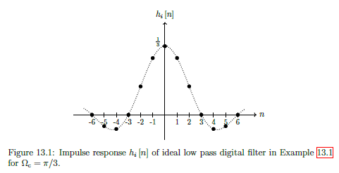
Practical Digital Filters
Good digital low pass filter will try to realise the (unrealisable) ideal response. Will try to do this with FIR filters (always stable, tend to have greater flexibility to implement different frequency responses).
- Need to induce a delay to capture most of the ideal signal energy in causal time, ie: use
- Truncate response to delay tolerance , such that for . Also limits complexity of filter: shorter = smaller order
- Window response, scales each sample, attempt to mitigate negative effects of truncation
Windowing
Window Method - design process: start with ideal and windowing infinite time-domain response to obtain a realsiable that can be implemented.
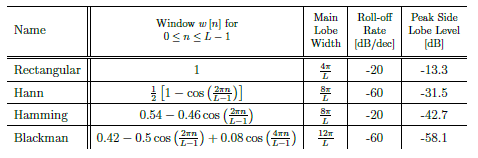
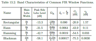
Windowing Criteria
- Main Lobe Width - Width in frequency of the main lobe.
- Roll-off rate - how sharply main lobe decreases, measured in dB/dec (db per decade).
- Peak side lobe level - Peak magnitude of the largest side lobe relative to the main lobe, measured in dB.
- Pass Band ripple - The amount the gain over the pass band can vary about unity and
- Pass Band Ripple Parameter, dB-
- Stop Band ripple - Gain over the stop band, must be less than the stop band ripple
- Transition Band -
Practical FIR Filter Design Example 13.2
See example...
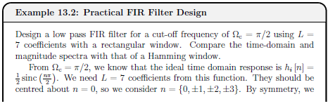
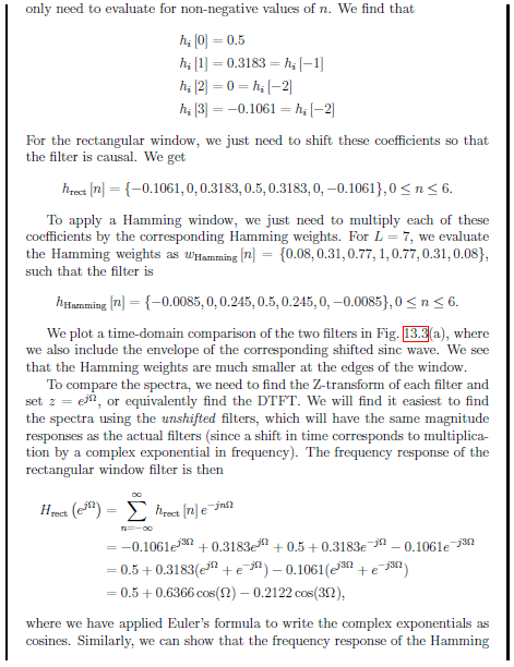
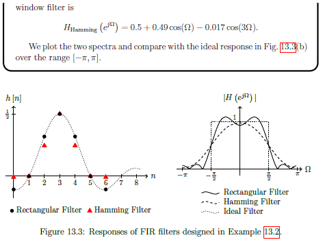
Specification for FIR Filters Example 13.3
See example...
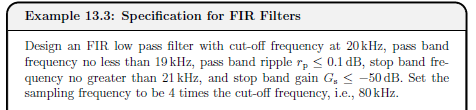
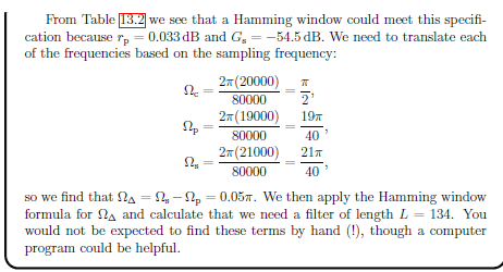
14 - Discrete Fourier Transform and FFT
Discrete Fourier Transform DFT
For
This is Forward discrete Fourier transform. (Not discrete time transform, but samples of it over interval
Explanation:
Discrete-time Fourier Transfomr (DTFT), takes discrete time signal, provides continous spectrem that repeats every . Defined for infinite length sequency , gives continous spectrum with values at all frequencies.
Digital often has finite length sequences. (Also inverse DTFT, uses intergration thus approximated). So assume sequence is length .
Sample spectrum . Repeats every , can sample over .
Take same number of samples in frequency domain as length of time domain signal.So evenly spaced samples of . (Aka bins)
Occur at fundemental frequency
Substitude into the DTFT.
For
Inverse DFT
Example 14.1 DFT of Sinusoid
See example
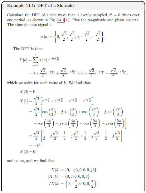
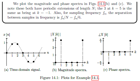
Zero Padding
Artificially increase the length of the time domain signal by adding zeros to the end to see more detail in the DTFT as DFT provides sampled view of DTFT, only see DTFT at frequencies.
Example 14.2 Effect of Zero Padding
See example
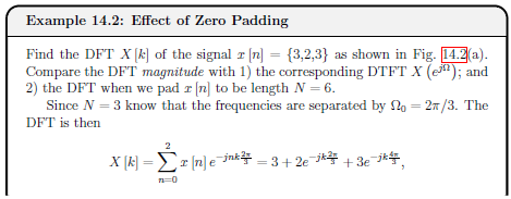
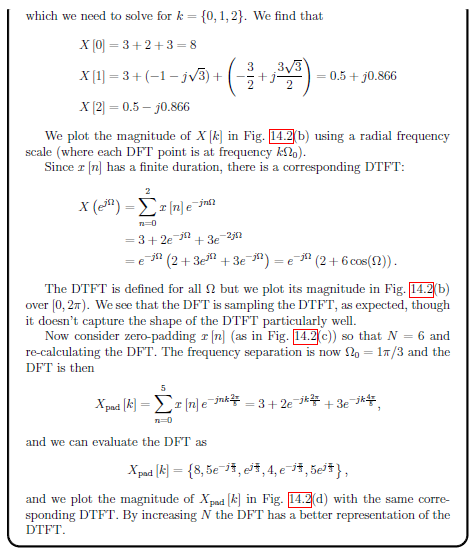
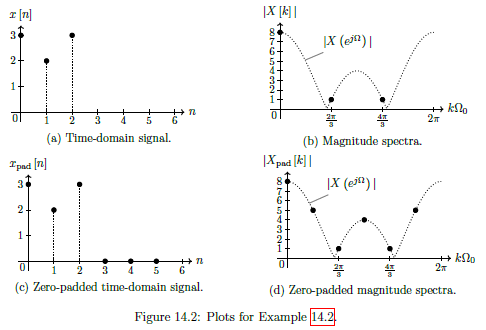
Fast Fourier Transform FFT
Family of alogrithms that evaluate DFT with complexity of compared to . Achieved with no approximations.
Details are beyond module, but can be used in matlab with fft function.
15 - Computing Digital Signals
This topic isn't examined as it is MATLAB
16 - Digital vs Analogue Recap
Aperiodic (simple periodic) continuous-time signal f(t)
Laplace, fourier transform.
- APeriodic (simple periodic) continuous time signal
- Convert to Laplace domain (s domain) via Laplace transform
- Which is the (continuous) Fourier transform.
- Fourier transform of the signal is its frequency response , generally defined for all
- Laplace and fourier transform, have corresponding inverse transforms, convert or back to
More Complex Continuous-time signal f(t)
Fourier series, multiples of fundamental, samples of frequency response.
- For a more complex periodic continuous-time signal f (t)
- Fourier series representation decomposes the signal into its frequency components at multiples of the fundamental frequency .
- Can be interpreted as samples of the frequency response ,
- which then corresponds to periodicity of over time.
- The coefficients are found over one period of .
Discrete-time signal f[n] (infinite length)
Z-Domain, Discrete-time fourier transform
- Discrete-time signal , we can convert to the z-domain via the Z-transform,
- Which for is the discrete-time Fourier transform DTFT.
- The discrete-time Fourier transform of the signal is its frequency response
- Repeats every (i.e., sampling in time corresponds to periodicity in frequency).
- There are corresponding inverse transforms to convert or back to
Discrete-time signal f[n] (finite length)
Finite Length N, convert to frequency domain (DFT), N points distributed over 2 pi (periodic)
- For discrete-time signal with finite length (or truncated to) N,
- Can convert to the frequency domain using the discrete Fourier transform,
- which is also discrete in frequency.
- The discrete Fourier transform also has N points distributed over and is otherwise periodic.
- Here, we see sampling in both frequency and time, corresponding to periodicity in the other domain (that we usually ignore in analysis and design because we define both the time domain signal and frequency domain signal over one period of length N).
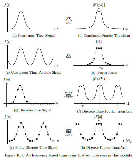
Stability
S-domain: negative real component, Z domain: poles within unit circle.

Bi-Linearity
Not core module content.
17 - Probabilities and random signals
Random Variable
A quantity that takes a non-deterministic values (ie we don't know what the value will be in advance).
Probability Distribution
Defines the probability that a random variable will take some value.
Probability Density Function (PDF) - Continuous random variables
For a random variable , take values between and (could be ), is the probability that .
The integration of these probabilities is equal to 1.
Can take integral over subset to calculate the probability of X being within that subset.
Probability mass function (PMF) - Discrete random variables
For a random variable , take values between and (could be ), is the probability that .
The sum of these probabilities is equal to 1.
Can take summation over subset to calculate the probability of X being within that subset.
Moments
Of PMF and PDF respectively.
- , called the mean - Expected (average) value
- , called the mean-squared value, describes spread of random variable.
Often refer second order moments to as variance . mean-squared value, with correction for the mean
Standard deviation
Uniform Distribution
Equal probability for a random variable to take any value in its domain, ie over .
PDF continuous version:
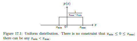
Discrete uniform distributions: result of dice roll, coin toss etc. Averege is average of min and max.
Bernoulli
Discrete probability distribution with only 2 possible values (yes no, 1 0, etc). Values have different probabilities, in general .
Mean: , Variance:
Gaussian (Normal) Distribution
Continuous probability distribution over , where values closer to mean are more likely.
Arguably most important continuos distribution as appears everywhere.
PDF is
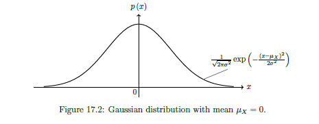
Central Limit Theorem (CLT)
Sum of independent random variables can be approximated with Gaussian distribution. Approximation improves with as more random variables are included in the sum. True for any probability distributions.
Independent Random Variables
No dependency on each other (i.e., if knowing the value of one random variable gives you no information to be able to better guess another random variable, then those random variables are independent of each other).
Empirical Distributions
Scaled histogram by total number of samples.
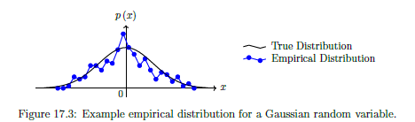
To observe behaviour that would match a PDF or PMF, require infinite number of samples. In practice can make histogram.
Random Signals
Random variables can appear in signals in different ways, eg:
- Thermal noise - in all electronics, from agitation electrons. Often modelled by adding gaussian random variable to signal
- Signal processing techniques introduce noise - aliasing, quantisation, non-ideal filters.
- Random variables can be used to store information, e.g., data can be encoded into bits and delivered across a communication channel. A receiver does not know the information in advance and can treat each bit as a Bernoulli random variable that it needs to estimate.
- Signals can be drastically transformed by the world (wireless signals obstructed by buildings trees etc) - Analogue signals passing through unknown system , which can vary with time etc
18 - Signal estimation
Signal Estimation
Signal estimation, refers to estimating the values of parameters embedded in a signal. Signals have noise, so can't just calculate parameters.
Linear Model
See equation
Polynomial terms,, linearity means y[n] must be linear function of unknown parameters.
EG:
- A,B are unknown parameters
- refers to noise - assume gaussian random variables with mean and varience - also assume white noise.
Write as column vector for each n.
Create observation matrix .
Since there are 2 parameters, matrix.
Can therefore be written as
With Optimal estimate :
Can write prediction:
Calculate MSE
Generalised Linear From
See equation
Where is a vector of known samples. Convenient when our signal is contaminated by some large interference with known characteristics.
To account for this in the estimator but subtracting by s from both sides.
Optimal estimate
See equation
Predicted estimate
See equation
Without noise.
Observation Matrix
See below
matrix where is the number of parameters, and is the number of time steps.
Each column is the coefficients of the corresponding parameter at the given timestamp (per row).
Mean Square Error (MSE)
See equation
Example 18.1
See example
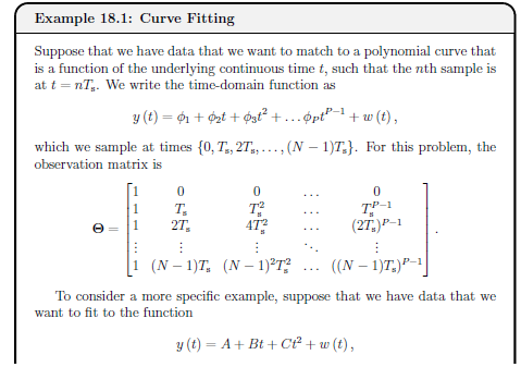
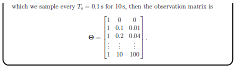
Example 18.2
See example
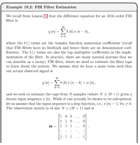
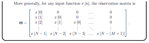
Linear Regression
AKA Ordinary least squares (OLS).
Form of observation matrix had to be assumed but may be unknown. If so can try different ones and find simplest that has best MSE.
Weighted Least Squares Estimate
Weighted least squares, includes a weight matrix W, where each sample associated with positive weight.
Places more emphasis on more reliable samples.
Good choice of weight :
Therefore resulting in:
Using equation, where W is the column vector of weights.
theta = lscov(Obs, y,W);
Maximum Likelihood Estimation (MLE)
See equation
Found by determining , maximises the PDF of the signal , which depends on the statistics of the noise .
Given some type of probability distribution, the MLE can be found.
MATLAB mle function from the Statistics and Machine Learning Toolbox.
19 - Correlation and Power spectral density
Correlation
Correlation gives a measure of time-domain similarity between two signals.
Cross Correlation
- is the time shift of sequence relative to the sequence.
- Approximation as signal lengths are finite and the signals could be random.
Example 19.1 - Discrete Cross-Correlation
See example
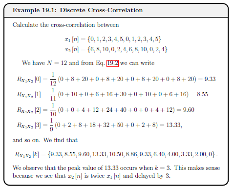
Autocorrelation
Correlation of a signal with itself, ie or
- Gives a measure of whether the current value of the signal says anything about a future value. Especially good for random signals.
Key Properties
- Autocorrelation for zero delay is the same as the signals mean square value. The auto correlation is never bigger for any non-zero delay.
- Auto correlation is an even function of or , ie
- Autocorrelation of sum of two uncorrelated signals is the same as the sums fo the autocorrelations of the two individual signals.
For and are uncorrelated,
Example 19.2 - Discrete Autocorrelation
See example
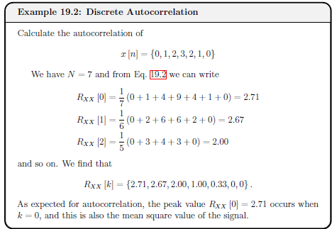
Example 19.3 - Correlation in MATLAB
See example
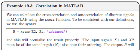
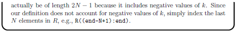
20 - Image Processing
Types of colour encoding
Binary (0, 1), Indexed (colour map), Greyscale (range 0->1), True Colour (RGB)
- Binary has value 0 and 1 to represent black and white
- Indexed each pixel has one value corresponding to pre-determined list of colours (colour map)
- Greyscale - each pixel has value within 0 (black) and 1 (white) - often write as whole numbers and then normalise
- True colour - Three associated values, RGB
But focus on binary and greyscale for hand calculations
Notation
See below
- follows same indexing conventions as MATLAB
ie: refers to vertical coordinate (row)
refers to horizontal coordinate (column)
is the top left pixel.
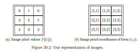
Digital Convolution
Example 20.1 - 1D Discrete Convolution
See example
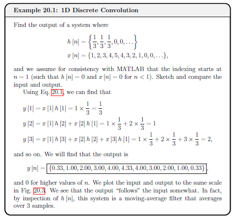
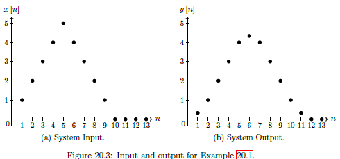
Example 20.2 - Visual 1D Discrete Convolution
See example
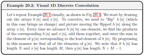
Image Filtering
Determine output y[i][j] from input x[i][j] through filter (kernel) h[i][j]
Filter (Kernel) = , assume square matrix with odd rows and columns so obvious middle
- Flip impulse response to get
- Achieved by mirroring all elements around center element.
- By symmetry, sometimes
- Move flipped impulse response along input image .
- Each time kernel is moved, multiply all elements of by corresponding covered pixels in .
- Add together products and store sum in output - corresponds to middle pixel covered by kernel
- Only consider overlaps between and where the middle element of the kernel covers a pixel in the input image
Edge Handling
Zero-padding and replicating
- Zero Padding Treat all off image pixels as having value 0. beyond defined image. Simplest but may lead to unusual artefacts at the edges of the image. Only option available for
conv2and default forimfilter. - Replicating the border - Assuming off image have same values as nearest element along edge of image. IE: Assume pixels at the outside corner take the value of the corner pixel
Kernels
Different types of kernels.
Larger kernels have increased sensitivity but more expensive to compute.
-
Values add to 0 = Removes signal strength to accentuate certain details
-
Values add to 1 = maintain signal strength by redistributing
-
Low Pass Filter - Equivalent to taking weight average around neighbourhood of pixel. Adds to 1
-
Blurring filter - Similar to low pass, but elements adds uo to more than 1, so washes out the image more
-
High Pass Filter - Accentuates transitions between colours, can be used as simple edge detection (important task, first step to detecting objects)
-
Sobel operator - More effective at detecting edges than high pass filter. Do need to apply different kernels for different directions. X-gradient = detecting vertical edges, Y-gradient = detecting horizontal edges
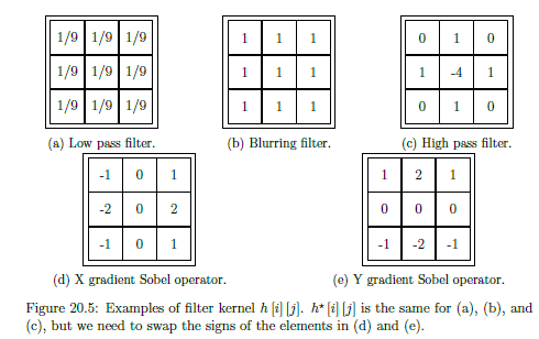
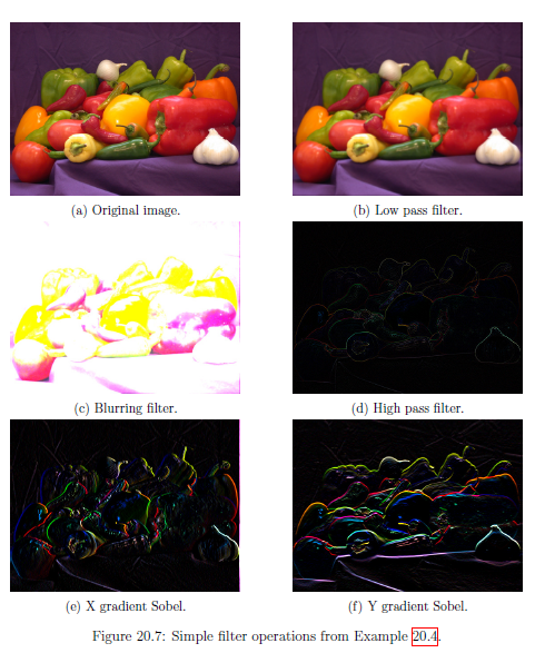
Example 20.3 - Image Filtering
See example
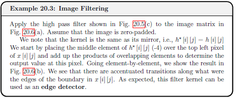
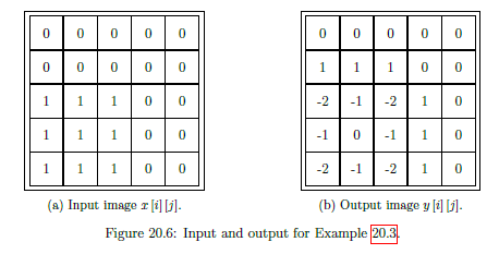
CS325
The notes here are very brief. Most notably they don't contain a lof of the detail of the methods/algorithms (below) needed for the exam.
Algorithms you need to know how to do on paper, by hand, in an exam
Because we just invented computers for fun, apparently.
- Lexing
- NFA/DFA stuff
- Parsing
- Grammar transformations
- Eliminating epsilon productions
- Eliminating left recursion
- Adding precedence
- Left factoring
- Removing ambiguity
- Computing
FirstandFollowsets - LL(1) parsing
- Constructing LL(1) parse table
- LR(k) parsing
- Shift-reduce
- Constructing set of LR(0) items
- Constructing LR(0) automaton
- Constructing LR(0) parse table
- Constructing SLR(1) parse table
- Grammar transformations
- Semantic analysis
- Annotating parse trees
- Constructing attribute grammars
- Constructing SDDs
- Constructing SDTs
- IRs
- Generating 3-address code for codegen stuff like addressing array elements and control flow
- Runtime Environments
- Working out access links/activation records and displays under different calling mechanisms
- Call-by-value
- Call-by-reference
- Call-by-name
- Copy-restore
- Garbage collection (less sure about this)
- Mark and sweep
- Pointer reversal
- Working out access links/activation records and displays under different calling mechanisms
- Optimisation
- Computing basic blocks of a program
- Dataflow analysis algorithms
- Reaching definitions
- Live variable analysis
- Available expressions
- Applying various optimisations to code
- Algebraic simplification
- Constant folding
- Unreachable block elimination
- Common subexpression elimination
- Copy/constant propagation
- Dead code elimination
- Reduction strength in induction variables
- Induction variable elimination
- Applying various transformations to loops
- Loop unrolling
- Loop coalescing
- Loop collapsing
- Loop peeling
- Loop normalisation
- Loop invariant code motion
- Loop unswitching
- Loop interchange
- Strip mining
- Loop tiling
- Loop distribution
- Loop fusion
- Codegen
- Instruction selection by replacing operations with sequences of assembly
- Using register and address descriptors
- Peephole optimisation
- Removing redundant loads/stores
- Removing jumps over jumps
- Algebraic optimisations
- Machine idioms
- Optimal codegen for expressions using Ershov numbers
- Including spilling to memory
- Instruction selection by tree rewriting
- Optimal tiling
- Graph colouring for register allocation
- Chaitin's algorithm - graph colouring heuristic
- Including spilling to memory
- Instruction selection by replacing operations with sequences of assembly
Lexing
We want to transform a stream of characters into a stream of tokens (token name, attribute value)
- A lexeme is the sequence of chars from source code
- A Regex is formal notation for a recogniser
- Recognisers are represented as finite automata
- - finite set of states in the recogniser along with error state
- is finite alphabet used by recogniser
- is transition function
- Maps states and characters to next state
- is the start state
- Set are accepting states
- An alphabet is a finite set of symbols
- String is sequence of symbols from alphabet
- Language is set of strings over the alphabet
- Defined using grammars
- We want to check if string on alphabet is a member of language
- Use a recognising automaton
- Diagrams are large, use regex to express
- Use a recognising automaton
- A language defined by a regex is the set of all strings that can be described by that regex
Tokenising
- Construct a regex matching all lexemes for all tokens
- Union of regexes for the token classes gives a regex that defines a language
- Given an input sequence of characters, want to check if some number of characters belong to the language
- Gor check if is in
- If true then we remove that string as a token and continue
- Always select the longer sequence - maximal munch
- If more than one token matches use the token class specified first
- If no match then error
- Can build a scanner from regex
- Require simulation of a DFA
- Thompson’s construction goes from NFA -> RE
- Subset construction builds a DFA that simulates an NFA
- Hopcroft’s algorithm minimises a DFA
- Kleene’s contruction dervices an RE from a DFA
- NFAs allow transitions on the empty string
- States may have multiple transitions on the same character.
- Can combine multiple FAs by just joining them with epsilon transisions
- DFAs only have a single transition on the each character from each state
- No epsilon transitions
- Can simulate any NFA
Thompson's Construction - RE to NFA
- Use a template for building an NFA that corresponds to
- A single letter regex
- Transformation on NFAs that models the effect of regex operators
- Combine fragments using epsilon transitions
- Take into account precedence
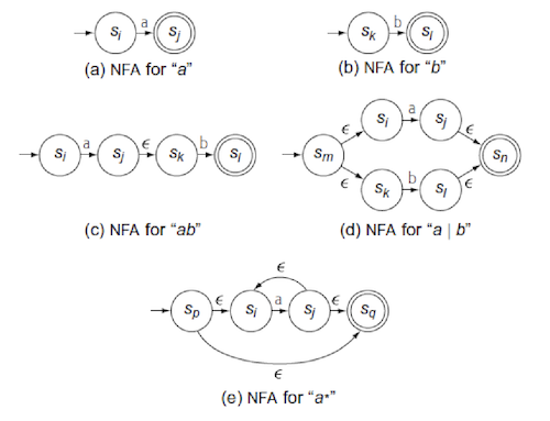
Subset Construction - NFA to DFA
Convert NFA to DFA to make it easier to simulate.
- Combine states based on epsilon transitions to eliminate them
- Create subset of states, then only consider transitions between subsets
- Set of states that can be reached from some state along only epsilon transitions is the epsilon closure of
Where there are several possible choices of next state, take all choices simultaneously and form a set of the possible next states. This set of NFA states becomes a single DFA state.
Hopcroft's algorithm - Minimising a DFA
Some states can be merged - partition states into groups of states that produce the same behaviour on any input string.
- Start by partitioning into accepting and non-accepting states
- Consider each subgroup
- Partition into new subgroups such that two states and are in the same subgroup iff for all input symbols , and have transitons on into the same group
- Replace group with new partitioning
- Keep going until convergence
Syntax Analysis
- Take a stream of words and parse it to check it’s correct
- Builds a parse tree
- If invalid then produce a syntax error
Context Free Grammars
- CFGs are formal mechanism for specifying syntax of source language
- Parsers parse text according to a grammar
- LL(1) top-down recursive descent
- LR(1) bottom up, canonical LR(1), LALR parser
- CFGs -
stmt -> if (expr) stmt else stmt- Four components
- Set of terminal symbols
- Set of nonterminal symbols
- One of the terminals is a start symbol
- Set of productions for nonterminals
- A grammar derives a sentence
- Parsing is the process of figuring out if a sentence is valid
- Rewrite expressions using grammar
- Four components
Parse Trees
- Parse tree represents derivation as graph
- Terminals at leaves, nonterminals as nodes
- In order gives input, postorder gives evaluation
- Right and leftmost derivations can give different results - grammar is ambiguous
- Bad property for a program to have
- Want to be able to rewrite them to be unambiguous
- Cannot be done automatically
- Also want to give correct mathematical precedence in parse tree
- Create a non-terminal for each level of precedence
- Isolate corresponding part of grammar
- Force parser to recognise high precedence subexpression first
Top-down Parsing
Top-down parsing starts at the root and grows the tree toward leaves.
- At each step, select a node for some nonterminal and extend it with a subtree that rewrites the nonterminal
- Always expand leftmost fringe of tree
- If choose wrong nonterminal parser must backtrack
- Expensive way to discover errors
Grammar scan be transformed to make them top-down parsable:
- Eliminate left recursion
- A grammar is left-recursive if it has a nonterminal such that there is some derivation
- The nonterminal at the head is the leftmost symbol of the body
- Topdown parsers cannot handle this
- Can easily eliminate direct left recursion
- Eliminate epsilon productions
- Eliminate cycles
- Given productions , replace productions by
- Indirect left recursion still a problem
- Need a more systematic approach
- Ommitted for sanity, see slide 54 onwards
- Symbol is nullable if it can be expanded with epsilon productions - can dissapear to an empty string
- Find nullable non-terminals, if nullable then create a new production by replacing it with epsilon
- Can increase grammar size
- A grammar is left-recursive if it has a nonterminal such that there is some derivation
Recursive descent parsers are programs with one parse function per nonterminal (see courserwork). Backtrack-free grammars are grammars that can be parsed by such parsers without having to backtrack.
- If top-down picks wrong the production it has to backtrack
- Can use a lookahead in input stream and use context to choose correct production
- set of is the set of terminals that begin strings derived from
- If is a terminal then
- For a nonterminal then is the complete set of terminal symbols that can appear as the leading symbol derived from
- If nonterminal is nullable then needs to be in first set
- set of terminals that can appear immediately to the right of
- is the symbols that can appear to the right of
- If is rightmost symbol in some sentinal form then
eofis in - For a production everything in except is in
- For or (where is nullable), everything in is in
- These are LL(1) grammars - can always predict the correct expansion at each point in the parse
- Choose production on a symbol if
- in
- is nullable and in
- Choose production on a symbol if
- Left factoring - convert grammar to have LL(1) property
- Rewrite nonterminals such that productions with common prefixes are factored into new nonterminals
- Table-driven LL(1) parsers are most common
- build first and follow sets
- the production of the form is in the table at if terminal or
eofis in OR if is nullable and is in - if table has conflicts then grammar is not LL(1)
Bottom-up parsing
Bottom-up parsing begins at the leaves and grows towards the root
- Identify a substring of the parse tree’s upper fringe that matches RHS of some production, build node for LHS and connect to tree
- Parser adds layers of nonterminals on top of leaves
- Reduces a string to the start symbol of the grammar
- Uses a stack that holds grammar symbols
- Shift reduce parsing:
- Parser shifts zero or more input symbols onto stack until ready to reduce a string
- Reduce into head of appropriate production
- Repeat until error detected or until stack contains start symbol and input is exhausted
- LR(k) parsers are most prevalent bottom up parsers
- L - scan Left to right, R - Rightmost derivation
- k can be 0, consider both 0 and 1 cases
- More powerful than LL(1) but harder
- Proper superset of predictive or LL methods
- For a grammar to be LR(k) must be able to recognise occurence of right side of production in a right-sentinal form, with k input symbols of lookahead
- Shift-reduce decisions
- LR parser makes shift-reduce decisions by maintaining state to keep track of where we are in parse
- Each state represents a set of items where item indicates how much of a production we have seen at a given point
- An item of a grammar is a production of , with a dot at some position of the body - this is an LR(0) item
- Collection of LR(0) items provides the basis for constructing a DFA called the LR(0) automaton that is used to make parsing decisions
- Steps:
- Create augmented grammar - add a $ for end symbol to indicate when it should stop parsing
- Compute closure set of items
- Every possible starting state of the automaton
- Compute GOTO functions for the set
- Defines transitions for automaton
- Can codify LR(0) automaton in a table to use for making shift-reduce decisions
- If a string of symbols takes the automaton from state
ito statejthen shift on the next symbol if statejhas a transision ona- Otherwise reduce
- Get shift/reduce conflicts in the table where do not have enough context on what to do
- If a string of symbols takes the automaton from state
- Steps:
- Can use SLR(1) parsing table to avoid conflits - use next symbol and set
- Uses same LR(0) items but uses an extra symbol of lookahead to make shift-reduce decisions
- Use set of nonterminal to determine if a reduction is correct
- All LR parsing is the same - table with input string and stack
- There are context-free grammars for which shift-reduce parsing does not work - either get shift/reduce or reduce/reduce conflicts
- More powerful parsers exist also
- LR(1) uses full set of lookahead symbols
- LALR parsers are based on LR(0) sets and carefully introduces lookaheads into LR(0) items
Semantic Analysis
A valid parse tree can be built that is gramatically correct, but the program may still be wrong according to the semantics of the language.
Syntax Directed Definitions
Attach rules to a grammar to evaluate some other shit
- Each nonterminal has a string-valued attribute that represents the expression generated by that nonterminal
- Symbol used for string concat
- Notation is attribute of
- Attributes can be of any kind - numbers, types, table references, strings
- It's a context free grammar with attributes and rules
- Can be done in a parse tree - use semantic rules for each node and transform tree in-order
- Gives annotated parse tree - has attribute values at each node
- Can be done in a parse tree - use semantic rules for each node and transform tree in-order
- Synthesised attributes are those where the value at the node is determined from attribute values of children
- Nonterminal at node is defined by semantic rule associated with production at
- Production must have at it’s head
- Has the desirable property that they can be evaluated during a single bottom-up traversal
- SDD with only synthesised attributes is called S-attributed - each rule computes attribute for nonterminal at the head from attributes taken from body
- Inherited attributes differ from synthesised attributes
- A nonterminal at a parse tree node is defined by a semantic rule associated with the production at the parent of
- Production must have as a symbol in it’s body
- Inherited attributes defined in terms of ’s parents, itself and siblings
- A nonterminal at a parse tree node is defined by a semantic rule associated with the production at the parent of
- SDDs have issues - makes grammar large
- Copy rules copy sets of info around the parse tree
- Increase space and complexity
- Can be avoided with a symbol table but that’s outside of this formalism
- Copy rules copy sets of info around the parse tree
Dependency Graphs
Determines evaluation order for attribute instances in parse tree
- Depict flow of information among attribute instances
- Edge from one attribute instance to another means that value of first is needed to compute second
- Gives order of evaluation - a topological sort of the graph
- If there are any cycles there are no topological sorts and SDD cannot be evaluated
- S-attributed grammars are those where every attributes are synthesised
- Can be evaluated in any bottom-up order
- Can evaluate using a post-order traversal
- Corresponds to order in which LR parse reduces production to head
- L-attributed grammars are those with synthesises and inherited attributes, but such that dependency graph edges can only go from left to right
Syntax Directed Translations
SDTs are based on SDDs - context free grammar augmented with program fragments called semantic actions
- Semantic actions can appear anywhere within production body
- SDTs more implementation oriented than SDDs - indicate order in which actions are evaluated
- Implemented during parsing without building parse tree
- Use a symbol table
- Denoted with braces placed around actions
$$refers to result location for current production$1, $2, ..., $nrefer to locations for symbols on the RHS of production
- To build SDT:
- Build parse tree ignoring actions
- For each interior node add additional children for the actions of the productions, from left to right
- Actions appear to right of productions in tree
- This gives postfix SDTs
- Do preorder traversal to evaluate
- Typically SDTs are done without building a parse tree
- Consider semantic actions as part of production body
- During parsing, actions is executed as soon as grammar symbols to the left have been matched
- Can have productions like
- If parse bottom-up then is performed as soon as appears on top of stack
- If parse top-down, is performed before we attempt to expand
- Postfix SDTs are always LR-parsable, always S-attributed with semantic action at end of production
- SDTs implementing L-attribute definitions are LL-parsable - pop and perform action when it comes to top of parse stack
Intermediate Representations
An IR is a data structure with all of the compiler's knowledge of a program
- Can be an AST or some sort of machine code (LLVM IR)
- Graphical IRs encode info in a graph
- Nodes, edges, lists, trees, etc
- Memory consuming
- Linear IRS are psuedo-code for some abstract machine on varying levels of abstraction
- Hybrid IRs combine elemends of both
- Use LLVM IR to represent blocks and a graph of the control flow between blocks
- Parse trees are an IR
ASTs
An abstract syntax tree retains the structure of a parse tree but ditches non-terminal nodes
- Can have a DAG to identify common sub-expressions
- Encodes redundancy - basic optimisation
- Must produce pure sub-expression
- Can use SDDs to construct a DAG
- Functions
leafandnodecreate a fresh node each time- If constructing DAG, then check identical node exists and if so then return that one
- Equivalence between nodes
node(op, left, right)established if node with labelopalready exists with sameleftandright, in that order
- Functions
- CFG models flow of control between basic blocks in program
- A Directed graph
- Typically used in conjunction with another IR
Linear IRs
Sequences of instructions executed in order. Like asm but with ✨abstraction✨.
One-address code
Models the behaviour of an accumulator machine or stack machine
- JVM, CPython do this
- Easy to generate and execute
Three-address code
Three-address code is expressions like i = j op k
- At most one operator per line
- Unravels multi-op expressions
- Compact and can be easily rearranged which is good for optimisation
- Most modern processors implement 3-address ops natively
- Can also be represented as a linearised syntax tree
- An address can be
- A name - pointer to symbol table entry
- A constant
- A compiler-generated temporary
- Instructions can be
- Assignment (unary)
- Assignment with a binary op
- Copies
- Jumps (conditional/unconditional)
- Procedure call
- Indexed copy (like index into arrays)
- Address and pointer stuff (think
*and&)
- Representing linear IRs
- Usually objects/records/structs with fields for operator and operands
- Quadruples have four fields -
op,arg1,arg2,result - Triples haver just
op,arg1,arg2- Refers to result by location in array of instruction
- Instructions cannot be easily re-arranged - requires changing references
- Indirect triples are similar but use a list of pointers to triples
- Can re-order by reordering instruction list without affecting triples themselves
- Different IRs exist on different levels of abstraction
- Structural IRs are usually high level
- Linear IRs usually lower level
- Can have a lower-level tree showing address calculations and registers n shit
- SSA is an IR that facilitates optimisations
- Names correspond uniquely to definition points in the code
- Each name is defined by a single operation
- Uses phi functions to combine definitions of two variables (ternary operators)
SDTs to generate IR
Actual program storage is runtime allocated, but relative addresses can be computed at compile time for local declarations
- From types we can determine storage size
- Type and relative address are saved in symbol table entry
- Dynamic types are handled by saving a pointer to runtime storage
- Can use an SDT to compute types and their widths
- Synthesised attributes for type and width of nonterminals
Can use an SDT to generate 3-address code for expressions too
- Array addressing is important when generating addresses
- Most languages number 0 to n-1
- Fortran numbers from 1 to n (cringe)
- Address of array element is
base + (i - low) * width - Can generalise to multiple dimensions
base + i1*w1 + i2*w2 + ... + ik * wk- Based on row- major layout - the way you’d expect
- Fortran uses column-major
- Can use this to generate grammar for array references - semantic actions for generating 3-address code to address arrays
- Most languages number 0 to n-1
Types are used by compilers to generate code and optimise
- Type synthesis builds type of expression from types of sub-exprs
- Type inference determines the type of an expression from the way it is used
- Type conversion can be explicit casts or implicit coercions
- Can use semantic actions for all of these
Control flow to IR is tied to translation of bools
- Used for flow of control and for logical values (and, or, not)
- Can use SDDs to evaluate boolean expressions and generate jumps and addresses for control flow
- May need to use backpatching
- Leave jump targets unspecified, do second pass to fill them in
A symbol table is a a data structure that used to hold info about source-program constructs
- May contain:
- Identifiers - data type, addresses, lexeme
- Arrays - dimensions
- Records/structs - fields and types
- Functions - number of params, types,
- Localises info - no need to annotate parse trees and makes stuff more efficient
- Scopes handled by having a separate symbol table for each scope
- Can use an SDT with semantic actions to generate a symbol table
Runtime Environments
We need to understand the compute or abstract machine we are generating code for.
Program Layout
- Compilers usually assume each executing program runs in own logical address space
- Mapped to physical addresses by OS
- Compiler is responsible for layout and manipulation of data
- Code goes at bottom of address space, followed by static storage, followed by heap (grows up towards stack), followed by stack (grows down towards heap)
- Storage layout influenced strongly by addressing constraints
- Alignment - 32 or 64 bit aligned?
- Compiler inserts padding in data types
- Static (compile time) and dynamic (runtime) memory are separate
- Stack stores static data local to procedure and sorts out call/return stuff via activation records
- Heap storage is for long lived stuff and may involve GC
- Stack allocation assumes execution is sequential and that control flow always return to point of call
- Allocation made possible by activations of procedure nesting in time
- Lifetimes of activations are properly nested
- Can use a tree to represent them
- Sequence of procedure calls corresponds to a pre-order traversal of activation tree
- Sequence of returns is a post-order traversal
- Live activations are those that correspond to a node and it’s ancestors
- Can use a tree to represent them
- Calls and returns managed by control stack - each live activation is a frame on the stack
- Top of stack is the currently active function
- Stack frame for a function contains
- Temporaries
- Local data
- Saved machine info (registers)
- Links: access, control, return
Procedure Calls
Calls are implemented by calling and return sequences - code inserted by compiler to push/pop from stack
- Caller evaluates function parameters and pushes
- Pushes return address
- Pushes caller’s local data and temps
- Callee saves register values and other status info
- Callee vs caller-svaes registers - designated per-register
- Caller-saves - save only registers that hold live variables
- Caller saves before function call
- May end up saving variables that callee does not use
- Callee-saves - save only registers that function actually uses in it’s body
- Save caller before re-using registers in own function body
- May end up saving registers that do not have live values
- Cannot avoid unnecessary saves
- Use a mixed strategy to optimise
- Designate some as caller and some as callee
- Caller-saves - save only registers that hold live variables
Variable Length Stack Data
Memory for data local to a procedure which has dynamic size (like C/C++ variable length arrays) may be stack allocated
- Avoids the expense of heap allocation
- Activation record does not hold storage for arrays - only a pointer to the beginning of each array
- Pointers are at known offsets from top-of-stack pointer
top- actual top of stack, points to where next activation record will begintop_sp- used to find local, fixed-length fields of current top activation record- Points to end of machine status field
- Both of the above can be generated at compile time
Scoping & Access Links
(cringe warning, this is confusing and terrible)
Accessing non-local stack data - mechanism for finding data within another procedure
- Static/lexical scope - find required data in enclosing scope
- Global vars have static storage - accessed through known addresses
- Dynamic scope/runtime binding - leave decision to runtime and look for closest stack frame which has required data
- Access links are pointers to activation records
- If procedure
pis nested within procedureq, then access link in any activation ofppoints to most recent activation ofq - Forms a chain from the activation record at top of stack to activations at lower depths
- If procedure
- Displays
- Access links inefficient if nesting depth large
- Faster access to nonlocals can be done using an array of pointer to activation records - a display
d[i]is a pointer to the highest activation record on the stack for any procedure at depthi- If procedure
pis executing and needs to access elementxbelonging to some procedureq- Look in
d[i] - Follow the pointer to get the activation record
- Variable is found at known offset
- Look in
- Compiler knows what
iis so can generate code for this
- Dynamic scope - new activation inherits existing bindings of nonlocal names
Parameter Passing
- Actual parameters are the ones passed into the call
- Formal parameters are those used in the function declaration
- l-values (memory location) vs r-values (expressions (not l-values))
- Call by value
- Treat formal parameters as a local name, storage for formal parameters is activation record, storage within stack frame
- Caller evaluates parameters and puts r-values into storage
- Can pass pointers to affect caller
- Call by reference
- Passes a pointer of the storage address of each parameter
- If lvalue, then lvalue is passed
- If rvalue then it’s evaluated and stored in a temporary and that lvalue passed
- Copy-restore
- Hybrid of the above two
- Copy-in copy-out
- Rvalues are passed as in call by value
- Lvalues are determined during call
- When control returns, current r-values copied back to lvalues computed earlier
- Call by name
- Procedure treated like a macro
- Cody substituted for caller, parameters literally substituted for formal params
- Local names of called procedure are kept distinct from names of calling procedure
- Inlining
- Similar to call by name
- Parameter passing becomes assignments
- Scoping managed correctly
- (usually) An optimisation to improve execution time
- Increases code size -> different instruction cache performance
- Similar to call by name
Memory Management
- Values outliving procedure that creates it cannot be kept in activation record
- Heap is used for data that lives indefinitely or for a while
- Memory manager is subsystem that allocates/deallocates space within heap
- Deals with
free/deletecalls - Java - GC
- Should be efficient
- Low runtime overhead
- Facilitate performance of programs
- Minimise heap space and fragmentation
- Deals with
- Fragmentaion caused by holes
- When freeing stuff, combine chunks
- Allocate memory in smallest holes possible - not good for spatial locality
- Next-fit placement - allocate in last split hole if enough space available
- Improves spatial locality as chunks allocated at same time are places together
- Manual allocation/deallocation (C/C++) is an issue - forget to free? fuck you.
- GC automatically reclaims free space by deleting unused objects
- Determine reachability of objects by starting from registers and following pointers
- Mark and sweep - mark reachable objects, then collect and free them all
- Coalesce gaps during sweep phase
- Requires memory to build list of dead objects but needs to be done when memory runs out
- Use pointer reversal - when a pointer is followed to get a reachable object it is reversed to point at it’s parent
- Gives an implicit stack to enable depth-first search of all reachable objects
Optimisations
Ideally compilers improve our code for us so it runs faster and uses less memory. Optimisations must preserve meaning however, so this is hard.
Basic Blocks
Basic blocks partition IR program into maximal sequences
- Flow of control enters only through first/last instructions in block
- No jumps in middle
- Flow of control leaves block at end
- Last instruction may branch
- Find branch instructions, identify targets, get basic blocks
- Blocks become nodes of control flow graph
- Compilers apply optimisations either locally, globally (entire function), or interprocedurally
- 1, 2 are common, 3 rare and has lower payoff
Local Optimisations
- Algebraic simplification - reduction in strength
- Replace complex ops with simple ones
- Replace muls with shifts
- Replace exponents with muls
- Constant folding
- Do operations at compile time
- Have to be careful when doing cross compilation due to different mathematical semantics on different architectures
- Eliminate unreachable basic blocks
- Makes code smaller and faster
- Commmon subexpression elimination
- Using SSA, two assignments with the same RHS compute the same value
- Copy propagation
- Using SSA, copies
u = vcan be changed for just substitutinguforv - No huge performance effect but facilitates constant folding and dead code elimination
- Using SSA, copies
- Dead code elimintation gets rid of code that does not contribute to a program’s result
Local optimisations do very little on their own but they typically interact. Compilers usually just do them until stuff stops happening.
Aliasing causes problems with optimisations - regions of memory that overlap
- Ones here assume no aliasing
- C allows to declare memory does not overlap with
restrictkeyword- Compiler does not check this
Global Optimisations
- Global common subexpression elimination - can be done accross blocks
- Knowing when values will be used next is useful for optimising
- Variables are live at a particular point in a program if it’s value is used in future
- To compute, look into future and work backwards
- Algorithm to compute live vars:
- For each statement
i: x = y op zdo:- Attach to
ithe current information in the symbol table regarding next use and liveness ofx, y, z - In symbol table, set
xto not live and no next use (x is assigned new value) - In symbol table, set
yandzto live and next uses ofyandztoi
- Attach to
- For each statement
- Liveness propagated backwards, against flow of control
- Variables are live at a particular point in a program if it’s value is used in future
- Data flow anlysis
- Derive info about flow of data along execution paths
- Dataflow values before and after statement are constrained by the semantics of that statement
- Relationship between before-after values is the transfer function
- Transfer function may describe dataflow in either direction
- - forward along execution path
- - backwards
- Easy for basic blocks - control flow value into a statement is the same as control flow value out of previous statement
- CFG edges create more complex constraints
- Transfer function of basic block is the composition of transfer functions of statements in block
- Constraints due to control flow between blocks can be rewritten substituting and for and
Reaching Definitions
- A definition of a variable is a statement that assigns to it
- The definition reaches a point if there is a point immediately following to such that is not killed along the path
- Statements may generate and kill definitions
- Transfer function of a definition can be expressed
- is set of definitions generate by statement
- is other definitions that kill
- is set of all definitions reaching , ie
- Transfer function of a definition can be expressed
- Composition of transfer functions like this is gen-kill form
- Extends to basic blocks with any number of statements
- Basic blocks also generate and kill sets of definitions
- Gen set is definitions that are downward exposed
- Kill set is union of all definitions killed by individual statements
- A definition may appear in both, gen takes precedence
- Iterative algorithm for computing reaching definitions
- is init to
- For each basic block other than entry
- Init to
- while there are any changes to - repeat until convergence
- = union of of predecessor blocks
- Used for optimisations - check if a definition if constant
Live Variable Analysis
We wish to know for variable and point if the value of at could be used along some path in the control flow graph starting at
- A variable is live if
- is used along some path starting at and there is no definition of along the path before the use
- A variable is dead if
- There is no use of on any path from to exit node or all paths from redefine before using it
- Need to look at future use of vars and work backwards
- Used for register alocation and dead code elimination
- Given the and set for a block, can relate live vars at beginning to live vars at end by
- Variable is live coming into a block if either:
- Used before redefinition in the block
- Is live coming out of the block and not redefined in the block
- Variable is live coming out of a block iff it is live coming into one of it’s successors
- Liveness is calculated backward starting from exit node
- Algorithm
- Assume all vars are dead at entry to a block
- Iterate starting from final node
- = union of all successor blocks in sets
- Repeat until convergence
Available Expressions
- An expression is available at a point if:
- Every path from entry node to evaluates before reaching
- There are no assignments to or after the evaluation but before
- Block kills expression if it assignns to or and does not recompute them
- Block generates expression if it evaluates them and then does not subsequently define them
- If an expression is available at use then there is no need to re-evaluate it - global common subexpression initialisation
- Expression is available at beginning of block iff available at the end of all predecessors
- Intersection is meet operator
Summary of dataflow analysis algorithms:
| Reaching Definitions | Live Variables | Available Expressions | |
|---|---|---|---|
| Domain | sets of definitions | sets of variables | sets of expressions |
| Direction | forwards | backwards | forwards |
| Transfer func | |||
| Boundary | |||
| Meet | union | union | intersect |
| Equations | |||
| Initalise |
Loop Optimisation
Loop optimisation is important to decrease overhead, exploit locality, increase parallelism, etc.
- In a loop a variable whose value is derived from number of iterations is called an induction variable
- Can be optimised by computing it with a single increment per loop iteration
- Where there are two or more induction vars may be possible to reduce to a single one
- Involves strength reduction
- When optimising loops, work inside-out
- Start with inner loops and then move to outer loops
- Loops are key, esp inner loops where lots of computation is done
- Can optimise loop by decreasing number of instructions in an inner loop
- Code motion - take an expression that yields same result independent of loop iteration and move it outside the loop
- Dependence is a relationship between two computations that constrains their execution order
- Control - determines control flow
- Data dependence - one computes something the other needs
- Flow dependence - one statement must be executed before another
- Antidependence - statement 1 reads a variable that is read by statement 2
- Has consequences for parallelisation
- Output dependence - two statements write to the same variable
- Have to describe dependence between iterations - loop carried dependencies
- Dependencies between two successive iterations
- Different classes of loop optimisations
- Loop restructuring
- Unrolling, coalescing, collapsing, peeling
- Dataflow-based loop transformations
- Loop-based strength reduction, induction variable elimination, invariant code motion
- Loop re-ordering
- Change the relative order of execution of iterations of a loop nest
- Expose parallelism and improve locality
- Loop interchange, strip mining, loop tiling, loop fusion
- Change the relative order of execution of iterations of a loop nest
- Loop restructuring
- Unrolling
- Replicate the loop body by an unrolling factor
u - Iterate by
usteps instead of 1 - Less overhead in loop conditions, longer basic blocks for better optimisations
- Replicate the loop body by an unrolling factor
- Coalescing
- Combine loop nest into a single loop
- Compute indices from resulting single induction var
- Improves scheduling on parallel machine
- Reduces overhead of loop nest
- Collapsing
- Less general version of coalescing in which dimensions of array is reduced
- Elimintates nested loops and multidimensional array indexing
- Best suited for loops that iterate over contiguous memory
- Peeling
- Small number of iterations removed from beginning/end and executed separately
- Removes dependence created by first or last few iterations
- Normalisation
- Converts all loops so that induction variable is initially 0 and always incremented by 1
- Exposes opportunities for fusion and simplifies analysis
- Invariant code motion
- Move computations outside loop where they do not change between iterations
- Reduce register pressure or avoid alu latency
- Unswitching
- Instead of having a conditional within a loop, have a loop within each branch
- Saves the repeated branching overhead
- Interchange
- Exchanges position of two loops in a perfect nest
- Perfect nest means the body over every loop contains only a loop
- Enables vectorisation, reduces stride, improves parallel performance
- Increase number of loop-invariant expressions in inner loop
- Exchanges position of two loops in a perfect nest
- Strip mining
- Adjust granularity of operation
- Similar to unrolling
- Choose number of independent computations in innermost loop of a nest
- Involves cleanup code in case number of iterations is not perfect multiple of strip
- Loop tiling
- Generalisation of strip mining in multiple dimensions
- Improve cache reuse by diving iteration space into tiles
- Critical for high performance in dense matrix multiplication
- Loop distribution
- Break a loop into many with same iteration space but subsets of statements of original loop
- Creates perfect loop nests
- Creates subloops with fewer dependencies
- Improves cache usage
- Reduce memory requirements
- Increase register reuse
- Loop fusion
- Opposite of the above
- Reduces loop overhead
- Increase instruction parallelism
Codegen
Want to take IR and output assembly that is semantically equivalent.
- The main tasks involved are:
- Instruction selection
- Register allocation
- Instruction ordering/scheduling
It is undecidable what the optimal program for any given IR is - we use heuristics.
Instruction selection
- Just translate each IR instruction to one or more machine code instructions
- Not very efficient
- Simple to implement but results in repeated loads/stores
- Keep track of values in registers to avoid unnecessary loads/stores
- Consider each instruction in turn
- Work out what loads are needed
- Generate code for loads
- Generate code for operation
- Generate code for stores
- Need to keep track of registers and memory locations for variables
- Register descriptor - (register, variable name) pairs
- Address descriptor - (variable name, location) pairs
- Location can be a register, memory address, stack location, etc
- Need some criteria for selecting registers
- If var currently in a register then no load needed
- If var not in a register then pick an empty one
- If y not in register and no empty ones then need to pick one to reuse
- Make sure that the value we reuse is either not needed or stored elsewhere
- Statement-by-statement codegen can be optimised with peephole optimisations
- Load/store pairs of the same instruction can be eliminated
- Only works if instructions are in same basic block
- Remove jumps over jumps
- useful in combination with constant propagation
- eg, removing debug info
- Flow control optimisations
- jumps-to-jumps can be eliminated
- Algebraic optimisations
- Eliminate instructions like
x = x + 0
- Eliminate instructions like
- Use of machine idioms
- target machine may have auto-increment addressing mode
- May have instructions that implement complex operations
- Load/store pairs of the same instruction can be eliminated
Optimal codegen from ASTs
- Can use the AST of an expression to generate an optimal code sequence
- Proven to generate shortest sequence of instructions
- Uses Ershov numbers
- Label any leaf
1 - Label of interior node with one child is the label of it’s child
- Label of an interior node with two children is
- Larger of the labels of it’s children if labels differ
- One plus the label of its children if labels same
- Label of node is the least number of registers in which expression can be evaluated using no stores of temporary results
- Label any leaf
- Can generate code from labelled expression tree
- Start at root of tree
- Registers used are
- For a node with label and two children with equal labels
gencode(right child)using base register- Result appears in
gencode(left child)using base register- Result appears in
- Generate instruction
OP
- To generate code for interior node with unequal labels
gencode(big child)using base register- result appears in
gencode(small child)using base register b- result appears in
- Evaluating expressions with insufficient register supply means you need extra memory
- Spill from registers into memory
- For interior node with label number of registers, work on each side of tree separately and store result in larger subtree
- Generate stores after code to eval registers for big child
Tree Rewriting
- Above algorithm works with RISC instruction sets but CISC instruction sets allow steps to be condensed into one instruction
- Treat instruction selection as a tree rewriting problem
- Machine instructions implement fragments of IR trees
- Match tree patterns with instructions
indoperator is dereferencing, is offset- Attempt to tile the subtree
- Tiles are set of tree patterns that correspond to legal machine instructions
- Cover the tree with non-overlapping tiles
- If template matches, matching subtree is replaced with replacement node of rule and machine instruction emitted
- Has it's issues
- Often multiple possibilities
- Best tiling corresponds to shortest sequence of instructions
- If none matches then process blocks
- Need to guard against possibility of single node being rewritten indefinitely
- Often multiple possibilities
- Optimal tiling - maximal munch
- Start at root
- Find largest tile that covers root node
- Generate that instruction
- Goto step 1
- Generates instructions in reverse order
- Optimum tiling - dynamic programming
- Bottom up rewrite system
- Omitted for sanity
Register allocation
Decide what to keep in registers and what in memory
- Efficient register use is important
- When code has more live values than registers, spill to memory
- this is costly
- Register allocation is NP complete
- Register assignment can be solved in polynomial time
- Can re-order instructions based on dataflow to optimise register assignment and reduce spill
Graph colouring
- Allocate based on liveness
- Works accross basic blocks
- Steps:
- Compute live variables for each point in program
- Generate an interference graph
- Each variable becomes a node
- If variables are live at the same time then make an edge connecting them
- They cannot be in the same register
- Colour the graph
- Nodes connected by edge cannot be the same colour
- A k-colourable graph uses no more than k registers
- NP hard too, use heuristics
- Algorithm to colour graph with colours - Chaitin’s algorithm
- Step 1:
- While has some node with neighbours less then
- Pick a node with less than neighbours
- Put on stack and remove from
- Repeat until is empty
- If all nodes removed then graph k-colourable, else no
- Step 2 - assign colours to nodes
- Start at top of stack
- Add node on stack top to graph including edges
- Pick a new colour
- Repeat until stack empty
- If colouring not found then have to spill to memory
- Will occur when each node has or more neighbours
- Pick candidate node for spilling and remove from graph, continue as before
- Have to insert loads/stores for spilled node
- Which one to spill? Any is fine but affects performance
- Spill those with most conflicts
- Spill those with few uses
- Avoid spilling in loops
ES3E6 - RF Electronics and Microwave Engineering
RF Semiconductors
Transmission Lines
A transmission line is a two port network that connects a source to a load
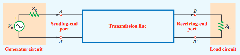
Modes
- Modes descibe the field pattern of propogating waves
- Can be found by solving Maxwell's equations in a transmission line
- In a transmission line, electric and magnetic fields are orthogonal to each other, and both orthogonal to the direction of propogation
- This is TEM (Transverse Electromagnetic) mode
- A TEM transmission line is represented by two parallel wires
- To reason about voltages and currents within it, we divide it into differential sections
- Each section is represented by an equivalent lumped element circuit
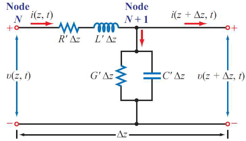
- - the combined resistance of both conductors per unit length, in
- - the combined inductance of both conductors per unit length, in
- - the combined capacitance of both conductors per unit length, in
- - the conductance of the insulation medium between the two conductors per unit length, in
The table below gives parameters for some common transmission lines
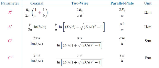
- Conductors have magnetic permeability and conductivity
- The insulating/spacing material has permittivity , permeability and conductivity
- All TEM transmission lines share the relations
- The constant propogation constant of a line
- is the attenuation constant (Np/m)
- is the phase constant (rad/m)
- The travelling wave solutions of a line are
- represents position along th eline
- represents the incident wave from source to load
- represents the reflected wave from load to source
We therefore have the characterisitic impedance of the TEM transmission line:
Both the voltage and current waves propagate with a phase velocity . The presence of the two waves propagating in opposite directions produces a standing wave.
The Lossless Transmission Line
In most practical situations, we can assume a transmission line to be lossless:
- , and
- Assume , so
- Therefore, as :
This then gives velocity and wavelength:
As the insulating material is usually non-magnetic, we have
Voltage Reflection Coefficient
Assume a transmission line in which the signals are produced by a generator with impedance and is terminated by a load impedance .
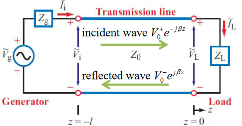
At any position on the line, the total voltage and current is:
At the load at position , the load impedance is:
Using this we can find an expression for the ratio of backwards wave amplitude and forward wave amplitude. We obtain the equation below, the voltage reflection coefficient
- for a lossless line is a real number, but may be a complex quantity
- In general, the reflection coefficient is also complex,
- Note that , always
- A load is matched to a line when , as then
- No reflection by the load
- If then , then
- Open circuit load
- If then , then
- Short circuit load
Standing Waves
The standing wave equation gives an expression for the standing wave voltage at position
The ratio of to is called the Voltage Standing Wave Ratio, or VSWR. Max occurs when , and min occurs when
Input Impedance of Lossless Lines
The input impedance of a transmission line is the ratio of the total voltage to the total current at any point on the line
- For a short circuit line ,
- For an open circuit line ,
The Smith Chart
The Smith chart is a graphical tool for analysing and designing transmission line circuits. It represents the reflection coefficient's complex plane.
The image below shows the the complex plane
- Point A is the reflection coefficient
- Point B is the reflection coefficient
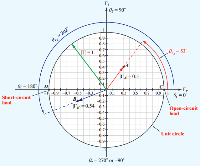
The Smith chart shows circles of constant normalised resistance , and constant normalised reactance , within the unit circle plane.
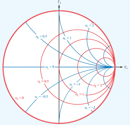
Given the normalised value of a load impedance , we can find the value of the corresponding reflection coefficient, and vice-versa.
Example
In the example below, point is plotted on the and lines, representing a normalised impedance of .
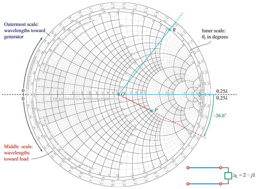
- The length of the line between the and the centre corresponds to the magnitude of the reflection coefficient
- The angle between the x axis and the point is
Phase Shifting
Based on the input impedance in terms of the reflection coefficient, we obtain
is the phase shifted reflection coefficient. at on a transmission line is equal to the reflection coefficient at the load (), shifted by :
This phase shift can be achieved on the Smith chart by maintaining constant magnitude, and decreasing the phase by the phase, corresponding to a clockwise rotation of an angle radians.
A complete rotation of radians corresponds to a change in length of . The outermost scale on the chart "wavelengths toward the generator" denotes movement on the transmission line toward the source, in units of wavelength.
Example
Point is a normalised load of at . If the load terminates a transmission line of length , what it's input impedance?
- Move clockwise by around a constant circle
- Read the smith chart at point to get
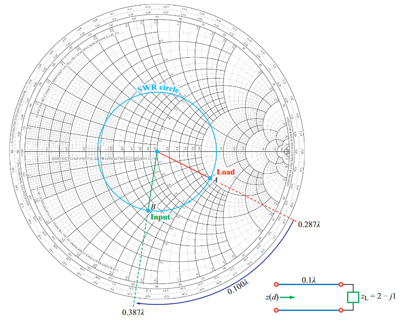
Admittance
For some problems, it is more convenient to work with admittances than with impedances
Normalised admittance is therefore:
- Rotation by on the SWR circle transforms into , and vice-versa
- circles become circles
- become circles
Example
Point represents a normalised load impedance of . Moving on the SWR circle by gives point , the corresponding normalised admittance of
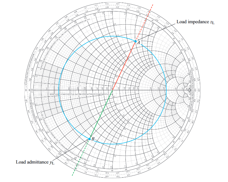
Narrowband Matching
A transmission line of characteristic impedance is matched to a load when : not incident waves upon the load are reflected back at the source. A matching network is used to achieve these conditions, placed between the load and the line. Examples of matching networks include
- The transformer
- A transmission line in series of length
- A capacitor/inductor in shunt
- A short circuit stub in parallel
Note that for lines of length , since , the input impedance of the line is equal to the load impedance and the line does not modify the impedance of the load to which it is connected.
Transformer
The input impedance of a line of length is
![]()
This eliminates reflections at to make .
$$ \Gamma = \frac{Z_{in} - Z_0}{Z_{in_} + Z_0} $$
At the frequency for which the transformer is a perfect , there is a perfect match, and . However, as we deviate from the match frequency, the performance degrades:
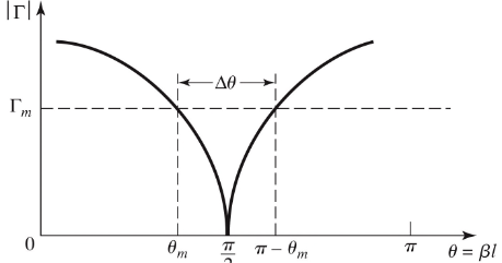
We use as an acceptable maximum reflection coefficent, for which the bandwith is defined:
Solving for from the above equations gives:
Assuming TEM lines, where is the designed frequency, we can then link with , the max/min frequency at which our match has an acceptable performance:
The fractional bandwith of a matching section (where is derived above):
The smaller the load mismatch, the larger the bandwidth.
Lumped Element Matching Networks
An L-secion uses two reactive elements to match a load impedance to a transmission line. If falls within the circle on the Smith chart, then the left configuration is used, else the right configuration is used.
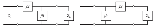
Let where (inside circle). For an impedance match:
Solving for and :
Two solutions are possible, and both are physically realisable with capacitors/inductors.
Conside the alternative where (outside circle):
Shunt Lumped Element Matching
We use a lumped element in parallel with the load to achieve matching as shown in the figure. As the element is in shunt, we work in the admittance domain.
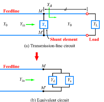
Assuming , the aim is at terminal to transform to , and to . Assuming and , the aim is to choose a length and value of to match of the feedline to , given by the sum of and .
Broadband Matching
Multi-section transformers can be used where a wider bandwith of matching is required than can be achieved by a single transformer.
Small Reflections
To derive such a transformer, we start with the theory of small reflections, applied to a single-section transformer. The incident wave will partially reflect and partially transmit at the interface, which will then reflect at the load, and then reflect again at the boundary, and so on.
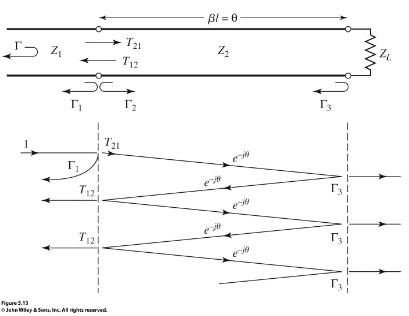
Summing the reflections/transmissions, the total reflection seen by the feedline is:
This is a geometric series, which sums to:
Multisection Transformer
Consider now a multisection transformer, which is just lots of small sections of transmission line of equal length
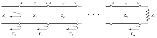
Making a few assumptions:
- Assume the differences between adjacent impedances are small
- Assume all increase or decrease monotonically
- Assume is real
- will be real and of the same sign
The total reflection coefficient is therefore:
Any desired value of can be synthesised by suitably choosing and .
The Binomial Transformer
We show how to realise such a transformer with a maximally flat total reflection coefficient, a binomial transformer.
For an -section transformer:
- Set the first derivatives of to 0 at the center frequency
- Provided by a reflection coefficient of the form
- Magnitude is then
- To determine , let
- Expression reduces to
- All sections are of 0 electrical length as
is expressed as a binomial series:
Because we assume are all small, we can approximate the characteristic impedances as:
To find the bandwith of the binomial transformer, let be the maximum tolerated reflection coefficient over the passband.
is the lower edge of the passband. Therefore:
And the fractional bandwith:
Rectangular Waveguides
Waveguides are just rectangular tubes full of air for transmission of power waves at high frequencies. Waveguides with a single conductor support either TE or TM waves, but not TEM waves.
- Modes define the properties of how a wave propagates through a guide
- Modes are defined by and
- Obtained through solving the wave equations for different boundary conditions
- Mode with lowest cutoff frequency is the dominant mode
- Dominant TM mode is
- Dominant TE mode is
TM Modes
Phase Constant
A wave is travelling inside the guide along the z-direction. It's phase factor is with:
Cutoff Frequency
Corresponding to each mode there is a cutoff frequency at which . A mode can only propagate if , as only then is real.
is the phase velocity of a TEM wave in an unbounded medium with parameters and .
Phase Velocity
Wave Impedance
is the intrinsic impedance of the lossless medium.
TE Mode
All the parameters are the same as for TM mode, except for wave impedance
The TE dominant mode, assuming where and are the width and height of the waveguide ,is with
Zigzag Reflections
For the mode, the field component can be expressed as the sum of two TEM plane waves, both travelling in the direction, but zigzagging between opposite walls of the waveguide. The phase velocity of these waves is and their direction is at angles. The phase velocity of their combination is that of the mode.
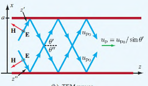
Table
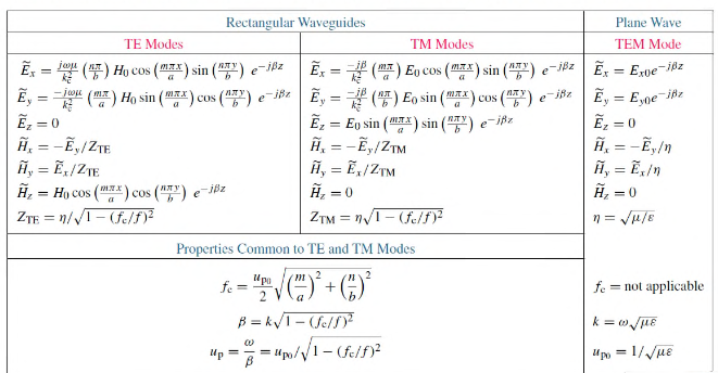
Coaxial & Microstrip Lines
Coaxial
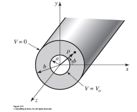
- The coaxial line is a waveguide
- Unlike the rectangular waveguide, coax supports the TEM mode, as well as higher order modes
- Field profiles for which can be found by solving the wave equations in cylindrical coordinates
- Using the cutoff frequency for the mode, the monomode frequency can be obtained
- The highest usable frequency before mode starts to propagate
- Cutoff wave number is approximated as
- , are the radii of inner and outer sheaths of cable
- Cutoff frequency found as
- Most common coax cables and connectors are 50 Ohm
- Air-filled coax line is 77 Ohm
- Max power capacity is at 30 Ohms
- 50 Ohms is the tradeoff between the two
- 75 Ohms used in TV systems
Microstrip Lines
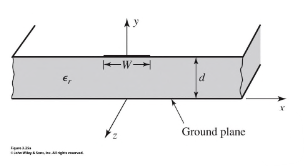
- Microstrips are a conductor of length printed on a thin, grounded dielectric substance of thickness and relative permittivity
- If there were no dielectric substrate, then we'd have a two wire TEM line with and .
- We don't
- The dielectric complicates the analysis
- It's almost-TEM, kind of a hybrid
- Some field lines are in the air region above the substrate, so no pure TEM wave
- Can approximate behaviour from quasi-static solutions
- is the effective dielectric constant of the microstrip
The effective dielectric constant can be interpreted as the dielectric constant of a homogenous medium that equivalently replaces the air and dielectric regions of the microstrip line
The characteristic impedance can be calculated as:
For a given and , we can also determine the ratio
Again considering the microstrip as a quasi-TEM line, we can determine the attenuation due to dielectric loss and conductor loss
Where is the surface resistivity of the conductor, and the loss tangent of the dielectric. For most substrates, .
Waveguide Discontinuities
Transmission lines often include discontinuities to perform an electrical function. Usually, these can be represented as equivalent circuits for analysis and design. Some common microstrip discontinuities and their equivalent lumped element circuits are shown below.

Striplines
A stripline is a planar transmission line used in microwave integrated circuits.
- Thin conducting strip of width between two wide conducting ground plates of separation ,
- Between the ground plates is filled with dielectric
- Supports usual TEM mode
- Can support higher-order modes, but can usually avoided by restricting spacing and geometry
Network Parameters
Impedance & Admittance Parameters
- Consider an N-port microwave network
- Forward and backward voltage and current waves can be defined for TEM waves
- Can define matrices of impedances(/admittances) to relate voltage and current port parameters to each other
- Ports may be any type of transmission line for a single propagating mode
- At a specified point on the port, a terminal place is defined
- Terminal planes provide a phase reference for wave phasors
- Equivalent incident and reflected voltage and current also defined
- At the terminal, total voltage and current are given by
- Assumes coordinate along which propagation occurs is zero at terminal
The impedance matrix relates these voltages and currents:
Can similarly define an admittance matrix
The two matrices are inverses of each other: . Both matrices relate total port voltages and currents.
can be found by driving port with current , open circuiting all other ports, and measuring the open circuit voltage at port
is the input impedance looking into port , and is the transfer impedance between ports and .
The admittance matrix parameters are found similarly:
- If a network is reciprocal (contains no active devices), then the matrix is symmetric
- For a reciprocal lossless network, all the or elements are purely imaginary
- for any and
Any two port network can be reduced to an equivalent or network:
Scattering Parameters
- Direct measurements of voltage and current become not that useful at high frequency because of waves
- The scattering matrix representation is more in line with the direct measurement of waves
- Provides a complete description of an -port network, relating incident and reflected waves on ports.
The S-matrix is defined
is found by sending port an incident wave and measuring at port the reflected amplitude . The incident waves on the rest of the ports are set to 0, meaning all ports are terminated in matched loads to avoid reflections.
- is the reflection coefficient looking into port
- is the transmission coefficient (gain) from port to
- The scattering matrix for a reciprocal network is symmetric
- The scattering matrix fro a lossless network is unitary
- Identity
Shifting Reference Planes
In the original network, the terminal planes are assumed to be at , where is measured along the lossless line feeding the port. The matrix with this set of planes is . If the new reference planes are defined , then we get a new scattering matrix defined . From travelling waves on a lossless line:
We can use this shift to define in terms of
Transmission (ABCD) Parameters
Practical microwave networks consist of a cascade connection of two or more 2-port networks. It is useful to define a 2x2 transmission, or ABCD matrix, for each 2-port network such that the transmission matrix of the cascade connection can be obtained as the product of the transmission matrices of the individual networks.

Note the sign convention, which has flowing into port 1, and flowing out of port 2.
If two networks are cascaded, ie network 1 outputs into network 2, the transmission matrix of the cascaded network is the product of the two individually
Some useful ABCD parameters for common networks are shown below
Port Parameter Conversion Table
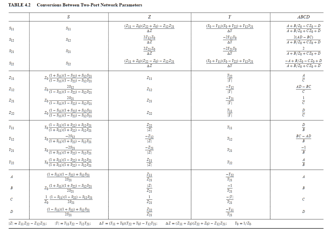
Filters
Filters are two port networks used to control frequency response.
Insertion Loss Method
We utilise the insertion loss method to design microwave filters.
We define a filter response by it's power loss ratio, the ratio of power available from the source to that delivered to the load.
The insertion loss (in dB) is then
As is an even function of , it can be expressed as a polynomial in :
By choosing coefficients of and , we can design filters with a specific frequency response.
Maximally Flat Response
Also known as binomial or Butterworth response. For a given filter order, it provides the flattest response in the passband. For a low pass filter of order with cutoff frequency :
- At the cutoff frequency, the power loss ratio is .
- If this is chosen as the -3 dB point then ,
- Usually the case
- If this is chosen as the -3 dB point then ,
- The first derivatives are zero at
- For , the insertion loss increases at a rate of dB/decade
Equal Ripple Response
A Chebyshev polynomial is used to specify the insertion loss:
- Results in a sharper cutoff
- Passband response will have ripples of amplitude , as oscillates between for
- determines the passband ripple level
- For large ,
- For , the power loss ratio is
- Increases at the same rate of dB per decade
- For , the power loss ratio is
- At any given , the power loss ratio is greater than that of the binomial filter for
Linear Phase Response
A linear phase response in the passband is important where signal distortion is to be avoided. A sharp-cutoff response is generally incompatible with a good phase response. Linear phase response can be achieved by:
- is the phase of the voltage transfer function of the filter
- is a constant
Normalised Design
We can normalise impedance and frequency values to simplify the design of filters.
Maximally Flat Response
Consider an LC circuit as shown below, with a source impedance of 1, a load impedance , and a cutoff frequency normalised to 1. The desired power loss ratio will be for .
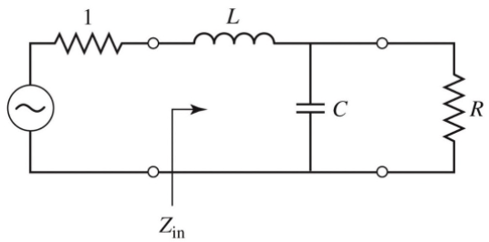
The power loss ratio of this filter can be derived from it's input impedance and reflection coefficient:
This equation solves to give , for the case .
The same process can be repeated for different values of to give the element values for the ladder-type circuits show. The values are numbred from source impedance to load impedance for a filter with reactive elements alternating between series and shunt connections.
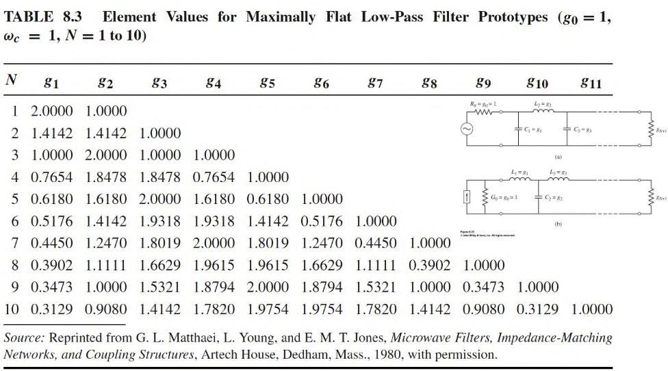
The graph shows attenuation vs normalised frequency for filter prototypes
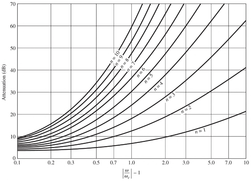
Equal Ripple Response
For Chebyshev polynomials, when is odd, and when even, so there are two cases for the power loss ratio depending on . Considering the same LC circuit shown above, for even it can be shown that is not unity, so there will be an impedance mismatch if the load has a unity impedance, which can be corrected with a transformer. For odd this is not an issue: it can be shown that .
The tables for equal ripple responses depend on the passband ripple level.
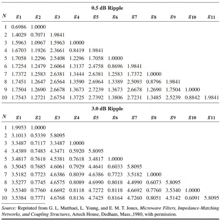
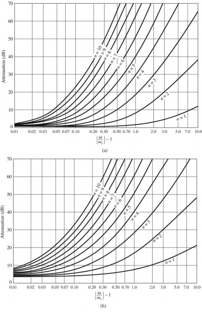
Scaling
In the prototype designs above, the source and load resistances are all unity. A source resistance of is obtained by multiplying all the impedances of the prototype design by
To change the cutoff frequency from unity to , replace by
Applying both impedance and frequency scaling, the new reactive element values are:
High Pass Transformation
The substitution is used to convert a low pass to high pass response. This maps and vice-versa.
The impedance and frequency scaling for mapping a normalised prototype to a high pass filter are:
Filter Implementation
Lumped elements are fine at low frequencies but usually don't work at RF. Richards' transformations can be used to convert lumped elements to transmission line sections:
The stub length of the lines is at with unity impedance.
The Kuroda identities can convert shunt to series. Each box represents a transmission line of the indicated characteristic impedance at length at . The inductors and capacitors represent short and open circuit stubs, respectively.
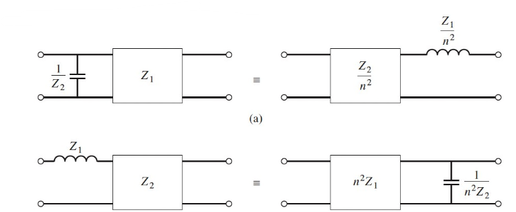
Stepped-Impedance Low Pass Filters
Low pass filters can be implement in microstrip using alternating sections of high and low impedance lines. For a low-pass filter prototype, the series indcutors can be replaced by high impedance line sections , and low impedance . The ratio should be as large as can possibly be fabricated. The lengths of the lines can then be determined from:
Where is the filter impedance, and and are the normalised element values from the prototype. To obtain the best response, the lengths should be evaluted at the cutoff frequency.
Power Dividers, Couplers & Resonators
Power dividers divider one input signal into two or more output signals. Power couplers take two or more inputs and combine them into a single output.
Wilkinson Power Divider
The equal split (3dB) Wilkinson power divider will be considered, although it can be designed to give arbitrary power division.
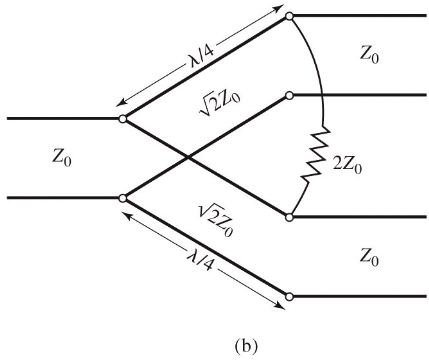
The circuit is formed of two lines of impedance , with a resisitor in shunt accross the two lines of impedance . The scattering parameters:
-
- at port 1, the input
-
- Ports 2 and 3 are matched for even and odd modes of excitation
-
- Symmetry due to reciprocity
-
- Due to short or open circuit at the bisection
Directional Coupler
A directional coupler is shown below
- Power supplied to port 1 is coupled to port 3
- The coupled port
- The remainder of the input power is delivered to port 2
- The through port
- No power is delivered to port 4
- The isolated port
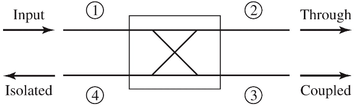
The quantities used to characterize a directional coupler:
- Coupling factor - the fraction of the input power that is coupled to the output port
- Directivity - a measure of the coupler's ability to isolate forward and backward waves
- Isolation - the measure of the power delivered to the uncoupled port
- Insertion loss - the power delievered to the output port
The quadrature hybrid directional coupler is a 3dB directional coupler with all ports matched, and input power divided evenly between ports 2 and 3. No power is coupled to port 4. The coupler is symmetrical, and any port can be used as the input/output ports.
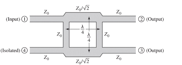
Resonators
RLC Resonators
Resonators at microwave frequency are similar to lumped element RLC circuits:
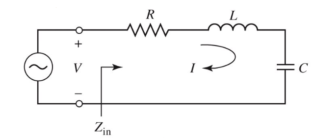
Input impedance:
Power delivered:
The resistors dissipates power , while the inductor and capacitor store energy and :
At the resonant frequency of , and
The quality factor of a resonant circuit is defined as the ratio of energy stored to energy loss:
measures the loss of the circuit: higher Q means higher loss. An external connecting network may introduce additional loss, so the of the resonator itself (the unloaded ) is:
The input impedance of the series resonator at a frequency , where is small:
A lossy resonator can be modelled as a lossless resonant frequency replaced by a complex effective resonant frequency .
When the frequency is such that , the real power delivered to the circuit is half that as of at . We use this to define the fractional bandwith as .
The same analysis can be done for a parallel RLC resonator. The properties of the two are compared in the table below
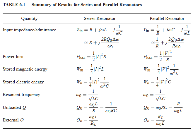
In general, resonators are coupled to other circuitry which gives a loaded . If we couple a resonant circuit to an external load and define , the external load, then:
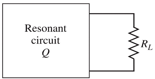
For a series RLC resonator, effective resistance is , and . In parallel, effective resistance is and
Transmission Line Resonators
Open Circuit line
A practical resonator that is often used in microstrip circuits is an open circuit length of transmission line of length , which behaves as a parallel resonator circuit. The input impedance is:
In practice, low loss transmission lines are used, so we can approximate . Using again for small near to the resonant frequency, we have:
At resonance, , the unloaded of this resonator is:
Gap-Coupled Microstrip Resonator
Consider a open-circuit microstrip gap-coupled to the end of a microstrip transmission line. The normalised input impedance is:
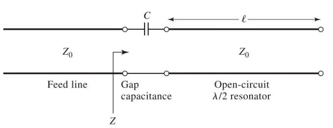
The resonant frequency occurs when , ie when
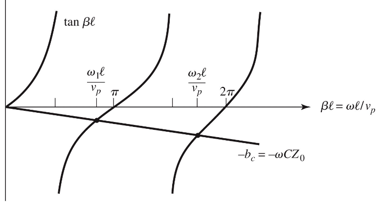
The first resonant frequency is close to the resonant frequency of the unloaded resonator, so we have . The coupling of the resonator to the feedline has the effect of lowering it's resonant frequency.
The presence of a coupling capacitor turns the uncoupled line from a parallel to a series RLC circuit near resonance. At resonance:
For critical coupling, :