Data Driven Models

• A system model can be developed from data describing the system
• Computational techniques can be used to fit data to a model

Modelling Approaches

White Box

• A white box model is a physical modelling approach, used where all the information about a system and its components is known.
• For example: "What is the voltage accross a 10 $\Omega$ resistor?"
  • The value of the resistor is known, so a mathematical model can be developed using knowledge of physics (Ohm's law in this case)
  • The model is then tested against data gathered from the system

Grey Box

• A grey box model is similar to white box, except where some physical parameters are unknown
• A model is developed using known physical properties, except some parameters are left unknown
• Data is then collected from testing and used to find parameted
• For example: "What is the force required to stretch this spring by $x$mm, when the stiffness is unknown"
  • Using knowledge, $F=Kx$
  • Test spring to collect data
  • Find value of $K$ that best fits the data to create a model
  • Final model is then tested
• Physical modelling used to get the form of the model, testing used to find unknown parameters
• This, and white box, is mostly what's been done so far

Black box

"Here is a new battery. We know nothing about it. How does it performance respond to changes in temperature?"

• Used to build models of a system where the internal operation of it is completely unknown: a "black box"
• Data is collected from testing the system
• An appropriate mathematical model is selected to fit the data
• The model is fit to the data to test how good it is
• The model is tested on new data to see how closely it models system behaviour

Modelling in Matlab

Regression

• Regression is predicting a continuous response from a set of predictor values
  • eg, predict extension of a spring given force, temperature, age
• Learn a function that maps a set of predictor variables to a set of response variables

For a linear model of some data $y=p_{1}x+p_0$:

• $y$ and $x$ are the predictor variables from the data set
• $p_1$ and $p_0$ are the unknowns to be estimated from the data
• Polynomial models can be used for more complex data

In Matlab

% data points
x = 0:0.1:1.0;
y = 2 * x + 3;
%introduce some noise into the data
y_noise = y + 0.1*randn(11,1)';

%see the data
figure;
plot(x,y_noise);
axis([0 1 0 5])

In matlab, the polyfit function (matlab docs) is used to fit a polynomial model of a given degree to the data.

• Inputs: x data, y data, polynomial degree
• Output: coefficients of model

P = polyfit(x,y_noise,1) % linear model
hold on;
plot(x,polyval(P,x),'r');

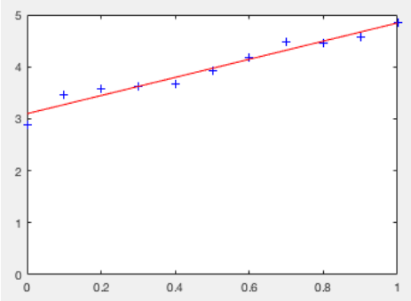
In the example shown, the model ended up as $y=1.7456x+3.0976$, which is close, but not exact due to noise introduced into the data.

Limitations

• Too complex of a model can lead to overfitting, where the model contains unwanted noise
• To overcome this:
  • Use simpler model
  • Collect more data