Filters

Filters are two port networks used to control frequency response.

Insertion Loss Method

We utilise the insertion loss method to design microwave filters.

We define a filter response by it's power loss ratio, the ratio of power available from the source to that delivered to the load.

$$P_{LR}=\frac{P_{inc}}{P_{load}}=\frac{1}{1-|\Gamma (\omega ){|}^2}$$

The insertion loss (in dB) is then

$$IL=10{\log }_{10}{P}_{LR}$$

As $|\Gamma (\omega ){|}^2$ is an even function of $\omega$, it can be expressed as a polynomial in ${\omega }^2$:

$$P_{LR}=1+\frac{M({\omega }^2)}{N({\omega }^2)}$$

By choosing coefficients of $M$ and $N$, we can design filters with a specific frequency response.

Maximally Flat Response

Also known as binomial or Butterworth response. For a given filter order, it provides the flattest response in the passband. For a low pass filter of order $N$ with cutoff frequency ${\omega }_c$:

$$P_{LR}=1+k^2{\left(\frac{\omega }{{\omega }_c}\right)}^{2N}$$

• At the cutoff frequency, the power loss ratio is $1+k^2$.
  • If this is chosen as the -3 dB point then $k=1$,
    • Usually the case
• The first $2N-1$ derivatives are zero at $\omega =0$
• For $\omega \gg {\omega }_c$, the insertion loss increases at a rate of $20N$ dB/decade

Equal Ripple Response

A Chebyshev polynomial $T_N(x)$ is used to specify the insertion loss:

$$P_{LR}=1+k^2{T}_N^2(\omega /{\omega }_c)$$

• Results in a sharper cutoff
• Passband response will have ripples of amplitude $1+k^2$, as $T_N(x)$ oscillates between $\pm 1$ for $|x|\le 1$
• $k^2$ determines the passband ripple level
• For large $x$, $T_N(x)\approx (2x{)}^{2N}/2$
  • For $\omega \gg {\omega }_c$, the power loss ratio is $(k^2/4)(2\omega /{\omega }_c{)}^{2N}$
    • Increases at the same rate of $20N$ dB per decade
• At any given $\omega$, the power loss ratio is $(2^{2N})/4$ greater than that of the binomial filter for $\omega \gg {\omega }_c$

Linear Phase Response

A linear phase response in the passband is important where signal distortion is to be avoided. A sharp-cutoff response is generally incompatible with a good phase response. Linear phase response can be achieved by:

$$\varphi (\omega )=A\omega \left[1+p{\left(\frac{\omega }{{\omega }_c}\right)}^{2N}\right]$$

• $\varphi (\omega )$ is the phase of the voltage transfer function of the filter
• $p$ is a constant

Normalised Design

We can normalise impedance and frequency values to simplify the design of filters.

Maximally Flat Response

Consider an LC circuit as shown below, with a source impedance of 1, a load impedance $R$, and a cutoff frequency normalised to 1. The desired power loss ratio will be $1+{\omega }^4$ for $N=2$.

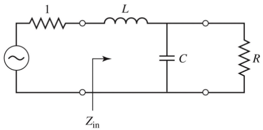
The power loss ratio of this filter can be derived from it's input impedance and reflection coefficient:

$$P_{LR}=\frac{|Z_{in}+1{|}^2}{2(Z_{in}+Z_{in}^{\ast })}=1+{\omega }^4$$

This equation solves to give $L=C=\sqrt{2}$, for the case $N=2$.

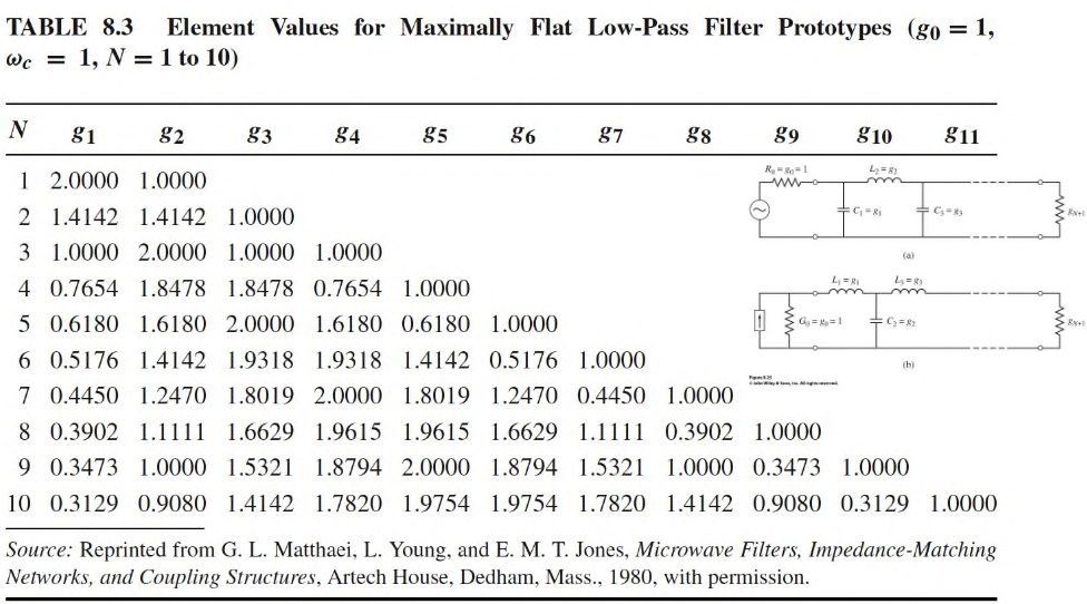
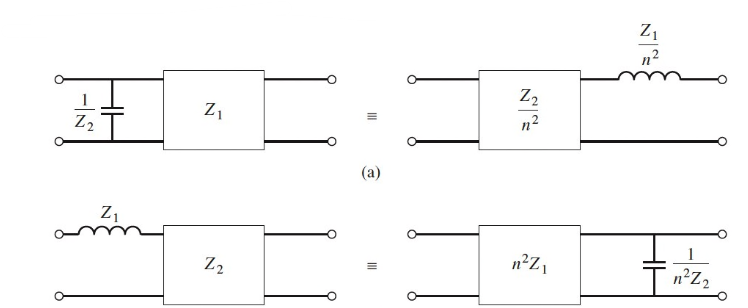
The same process can be repeated for different values of $N$ to give the element values for the ladder-type circuits show. The values are numbred from $g_0$ source impedance to $g_{N+1}$ load impedance for a filter with $N$ reactive elements alternating between series and shunt connections.

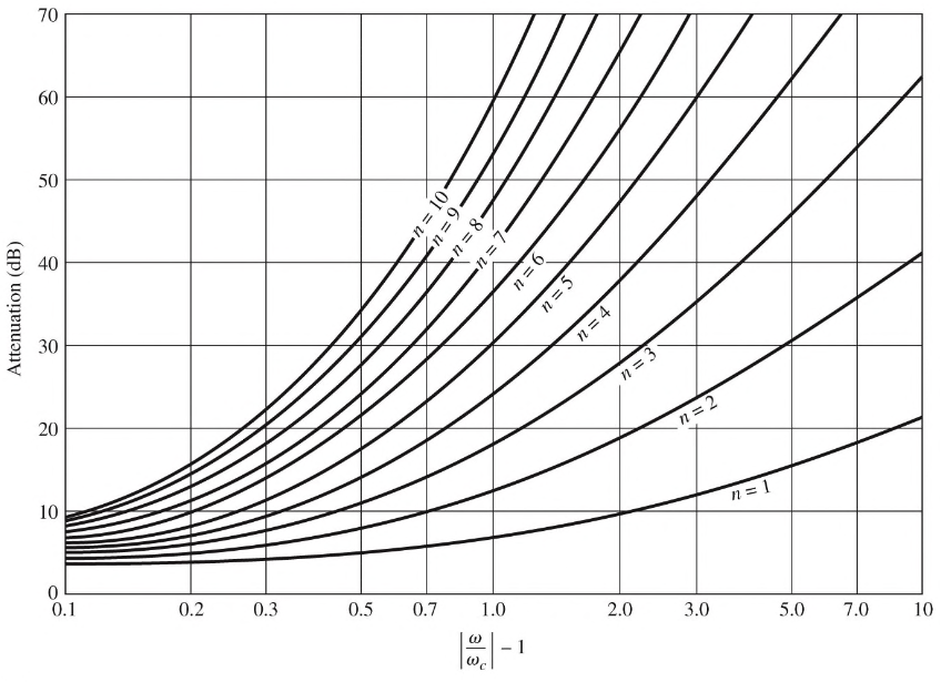
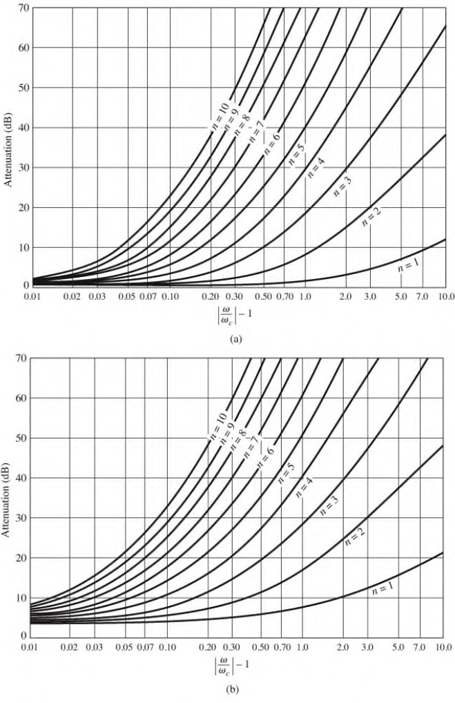
The graph shows attenuation vs normalised frequency for filter prototypes

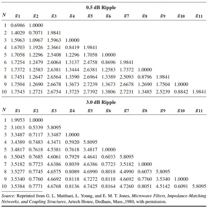
Equal Ripple Response

For Chebyshev polynomials, $T_N(0)=0$ when $N$ is odd, and $T_N(0)=0$ when even, so there are two cases for the power loss ratio depending on $N$. Considering the same LC circuit shown above, for even $N$ it can be shown that $R$ is not unity, so there will be an impedance mismatch if the load has a unity impedance, which can be corrected with a $\lambda /4$ transformer. For odd $N$ this is not an issue: it can be shown that $R=1$.

The tables for equal ripple responses depend on the passband ripple level.

Scaling

In the prototype designs above, the source and load resistances are all unity. A source resistance of $R_0$ is obtained by multiplying all the impedances of the prototype design by $R_0$

$$L^{\prime }=R_{0}L{C}^{\prime }=C/R_0{R}_s^{\prime }=R_0{R}_L^{\prime }=R_0{R}_L$$

To change the cutoff frequency from unity to ${\omega }_c$, replace $\omega$ by $\omega /{\omega }_c$

Applying both impedance and frequency scaling, the new reactive element values are:

$$L_k^{\prime }=\frac{R_0{L}_k}{{\omega }_c}{C}_k^{\prime }=\frac{C_k}{R_0{\omega }_c}$$

High Pass Transformation

The substitution $\omega \leftarrow (-{\omega }_c/\omega )$ is used to convert a low pass to high pass response. This maps $\omega =0\to \pm \infty$ and vice-versa.

The impedance and frequency scaling for mapping a normalised prototype to a high pass filter are:

$$C_k^{\prime }=\frac{1}{R_o{\omega }_c{L}_k}{L}_k^{\prime }=\frac{R_0}{{\omega }_c{C}_k}$$

Filter Implementation

Lumped elements are fine at low frequencies but usually don't work at RF. Richards' transformations can be used to convert lumped elements to transmission line sections:

$$j{X}_L=jL\tan (\beta l)j{B}_c=jC\tan (\beta l)$$

The stub length of the lines is $\lambda /8$ at ${\omega }_c$ with unity impedance.

The Kuroda identities can convert shunt to series. Each box represents a transmission line of the indicated characteristic impedance at length $\lambda /8$ at ${\omega }_c$. The inductors and capacitors represent short and open circuit stubs, respectively.

$$n^2=1+Z_2/Z_1$$

Stepped-Impedance Low Pass Filters

Low pass filters can be implement in microstrip using alternating sections of high and low impedance lines. For a low-pass filter prototype, the series indcutors can be replaced by high impedance line sections $Z_0=Z_h$, and low impedance $Z_0=Z_l$. The ratio $Z_h/Z_l$ should be as large as can possibly be fabricated. The lengths of the lines can then be determined from:

$$\beta l=\frac{L{R}_0}{Z_h}\beta l=\frac{C{Z}_l}{R_0}$$

Where $R_0$ is the filter impedance, and $L$ and $C$ are the normalised element values from the prototype. To obtain the best response, the lengths should be evaluted at the cutoff frequency.